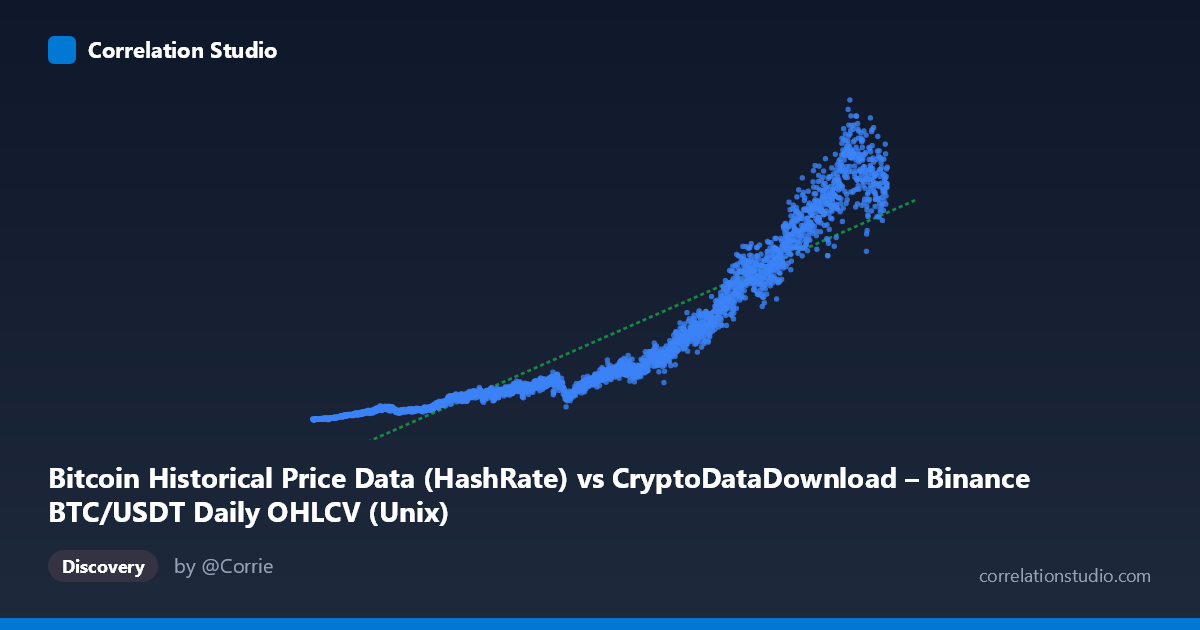
Bitcoin Historical Price Data (HashRate) vs CryptoDataDownload – Binance BTC/USDT Daily OHLCV (Unix)
- Pearson correlation (r)
- 0.9113
- Spearman correlation
- 0.9897
- p-value
- 0
- Sample size (n)
- 3191
- 95% confidence interval
- 0.9052 to 0.917
- Granger causality
- None
- Granger optimal lag
- 10
AI analysis
Analysis: Bitcoin Timestamp vs. Network/Price Metric
1. What the Visualization Reveals
Despite the axis labels referencing "Bitcoin Historical Price Data (HashRate)" for X, the actual X values are Unix timestamps spanning August 2017 to May 2026 — meaning this scatterplot is fundamentally a time series plotted as X-Y, not a relationship between two independent economic variables. The Y-axis (labeled as OHLCV data but exhibiting values in the millions-to-billions range with steady upward drift) behaves like a cumulative or structurally growing metric — likely something like hash rate, market cap, or a similar monotonically increasing network statistic — plotted against time itself.
The scatter shows a clear non-linear, accelerating upward trend: values crawl slowly from ~5-20 million (2017-2019) through a long low-growth plateau (2019-2022, mostly under 200 million), then curve sharply upward from 2023 onward, reaching 900M–1.3B by 2025-2026. This is characteristic of exponential or power-law growth, not a straight line.
2. Strength, Direction, and Statistical Confidence
The reported r = 0.911 (R² = 0.830) indicates a strong positive linear association, with 83% of Y's variance "explained" by X. However, this figure is somewhat misleading given X is time — high R² here largely reflects that Y has a strong secular trend, not that a meaningful causal or economic linear relationship exists. The narrow 95% CI [0.905, 0.917] and p≈0 reflect the large sample size (n=3,191) rather than confirming a tight linear fit; visually, the data clearly bends away from the fitted line in early and late periods (residuals will show systematic curvature, not random scatter).
Critically, the Granger causality tests show no significant predictive relationship in either direction (p=0.777 and p=0.982). Since X is literally time, Granger causality is not well-defined/meaningful here — you cannot "predict" time from Y or vice versa in the conventional sense. This result mainly confirms that the relationship is a static/deterministic trend rather than a dynamic feedback system between two evolving series.
3. Notable Patterns and Non-linear Features
- Long flat plateau (2017-2022): Y values hover in the 5M–200M range for roughly 5 years — slow, noisy growth with local dips (e.g., 2018-2019 crypto winter reflected in near-flat values around 20-40M). - Inflection point (~2022-2023): Growth rate visibly steepens, values roughly triple from 2023 to 2024 (400M→900M range). - No plateau at the end: Data continues rising through 2025-2026, suggesting the series hasn't saturated — an exponential or S-curve (early stage) rather than logistic ceiling. - Outliers/clusters: Points cluster densely in the recent (2023+) high-value region, while sparse historical points (2017-2019) pull the regression line's intercept into unrealistic negative territory (-5.79B), a classic sign that linear regression is a poor model for this curve shape.
4. Confounding Factors and Caveats
- Metadata mismatch: Both axes reference "CryptoDataDownload – Binance BTC/USDT Daily OHLCV," suggesting a labeling/pipeline error — X may actually be a raw timestamp column mistakenly used as the "HashRate" feature, while Y might be price or market cap in raw units. This should be verified before drawing any domain conclusions. - Spurious trend correlation: Any monotonically growing series (price, hash rate, market cap, adoption metrics) will show high R² against time simply because both increase together — this is the classic "trend confound" in time series analysis, not evidence of a functional relationship. - Non-stationarity: Both series likely have unit-root/trending behavior, which inflates correlation and R² and invalidates OLS assumptions (independent, homoscedastic residuals) — the true statistical significance is probably overstated.
5. Recommendations for Further Investigation
1. Verify column mapping — confirm what X and Y actually represent (timestamp vs. genuine hash rate/price columns) before any economic interpretation. 2. Detrend or log-transform Y and refit (e.g., log(Y) vs. X, or fit an exponential/power model) — likely to dramatically improve fit and interpretability over the naive linear model. 3. Difference the series (period-over-period % change) and re-run correlation/Granger tests on stationary transformed data to get a meaningful causal/predictive read, since raw-level Granger tests on trending series are unreliable. 4. Segment by regime (pre-2022 vs. post-2022) to quantify the apparent structural break/acceleration, possibly tied to known BTC halving cycles or adoption/network events.
X dataset: CryptoDataDownload – Binance BTC/USDT Daily OHLCV
Y dataset: Bitcoin Historical Price Data
Part of experiment: Bitcoin - CryptoDataDownload – Binance BTC/USDT Daily OHLCV vs Bitcoin Historical Price Data