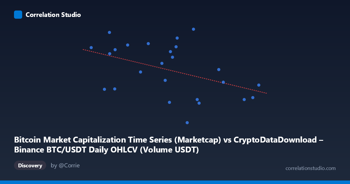
Bitcoin Market Capitalization Time Series (Marketcap) vs CryptoDataDownload – Binance BTC/USDT Daily OHLCV (Volume USDT)
- Pearson correlation (r)
- -0.4381
- Spearman correlation
- -0.3962
- p-value
- 0.028474
- Sample size (n)
- 25
- 95% confidence interval
- -0.7103 to -0.052
- Granger causality
- None
- Granger optimal lag
- 6
AI analysis
Analysis: Bitcoin Market Cap vs. Trading Volume (USDT)
1. What the Visualization Reveals
The scatterplot shows a modest negative relationship between Bitcoin's market capitalization and its USDT trading volume across this 25-day sample (late March to late April 2024). Points are widely scattered around the fitted regression line, with no tight clustering along the trend — visually confirming that market cap alone provides limited predictive power for volume in this window. The data cloud is roughly diffuse rather than forming a clear linear band, consistent with the weak-to-moderate correlation coefficient.
2. Strength, Direction, and Statistical Confidence
The correlation coefficient (r = -0.438) indicates a weak-to-moderate negative relationship: as market cap increases, volume tends to decrease slightly, and vice versa. However, r² = 0.192 means only 19% of the variance in volume is explained by market cap — the remaining 81% is driven by other factors entirely. The 95% confidence interval [-0.710, -0.052] is wide and asymmetric, reflecting substantial uncertainty from the small sample (n=25); the true relationship could range from strongly negative to nearly negligible. The p-value (0.028) is below the conventional 0.05 threshold, suggesting the correlation is statistically significant, but just barely — this is not strong evidence given the small sample size. Critically, the Granger causality tests show no significant predictive direction in either direction (X→Y: p=0.735; Y→X: p=0.773), meaning neither variable reliably helps forecast the other's future values based on past observations. This undercuts any temporal/causal interpretation — the contemporaneous correlation may be coincidental or driven by a shared external factor rather than one variable leading the other.
3. Notable Patterns and Outliers
Several points stand out: the highest Y-value (~1.409T) occurs at a mid-range X (~3.27B), while the lowest Y-value (~1.206T) occurs at a similarly mid-range X (~3.13B) — nearly identical market caps producing very different volumes, which itself illustrates the weak relationship. The extreme X-value (4.75B) sits at a below-average Y, contributing to the negative slope, but a nearby high-X point (4.61B) also has low Y, lending some support to the trend at the upper tail. No strong nonlinear curvature (e.g., clear quadratic or threshold pattern) is apparent — the scatter looks more like noise around a slightly tilted line than a structured nonlinear relationship.
4. Confounding Factors and Caveats
Several caveats limit interpretation: (1) Small sample size (n=25, ~3.5 weeks) makes correlation estimates unstable and highly sensitive to individual data points/outliers. (2) Market cap and volume both derive from price and supply, so they are not fully independent — price swings mechanically affect both variables simultaneously, potentially creating spurious correlation. (3) Time-series autocorrelation: daily financial data often exhibits serial dependence, which can violate assumptions of standard correlation tests and inflate apparent significance. (4) Omitted variables — macro factors (interest rate news, regulatory announcements, exchange-specific liquidity events, weekend/weekday effects) likely drive both market cap and volume independently, confounding the direct relationship. (5) The dataset spans a single month, which may not capture longer-term regime changes (bull/bear cycles) where the relationship could differ.
5. Actionable Insights
Given the lack of Granger causality and modest r², this relationship should not be used for predictive trading signals in its current form. Recommended next steps: (a) extend the time window to include more market cycles (bull/bear/sideways) to improve statistical power and robustness; (b) test with returns/log-differences instead of levels to address potential non-stationarity, a common issue in financial time series that can distort both correlation and Granger tests; (c) explore volume as a function of volatility or price change magnitude rather than raw market cap level, since volume often spikes with big price moves regardless of level; (d) incorporate additional exchanges or aggregate volume data to reduce Binance-specific noise. Until then, treat this correlation as suggestive but not actionable.
X dataset: CryptoDataDownload – Binance BTC/USDT Daily OHLCV
Y dataset: Bitcoin Market Capitalization Time Series
Part of experiment: Bitcoin - CryptoDataDownload – Binance BTC/USDT Daily OHLCV vs Bitcoin Market Capitalization Time Series