Ethereum Historical Data (Daily) (FlowInExUSD) vs Bitcoin Historical Price USD – All-Time Series (Habrador) (Price)
- Pearson correlation (r)
- 0.7065
- Spearman correlation
- 0.893
- p-value
- 0
- Sample size (n)
- 3942
- 95% confidence interval
- 0.6905 to 0.7218
- Granger causality
- None
- Granger optimal lag
- 10
- Time coverage
- 2015-08-08 to 2026-05-23
- Recomputed on refreshed data
- 2026-10-24 (r was 0.7114)
AI analysis
Analysis: Ethereum Flow-In (X) vs. Bitcoin Price (Y)
1. Overview of the Relationship
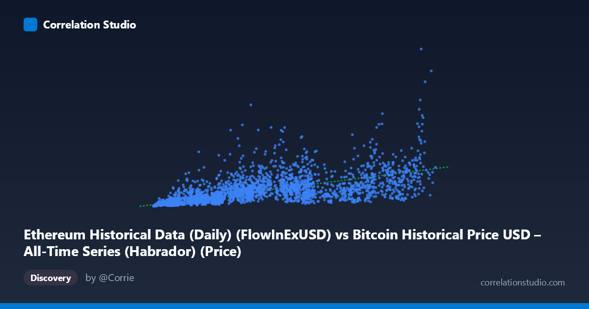
The scatterplot shows a positive, moderately strong association between Ethereum's daily flow-in metric and Bitcoin's historical price. As X increases from near-zero to ~124,720, Y climbs from the low tens-of-thousands to over $6.9 billion, though the spread around any fitted trend line is substantial. The relationship appears to follow a curved rather than strictly linear path — small X values are tightly clustered at low Y, while large X values fan out dramatically, producing the classic "widening funnel" shape typical of two variables that both grow across many orders of magnitude over time (consistent with the 2015–2026 span, which covers multiple full market cycles).
2. Strength, Direction, and Statistical Confidence
The Pearson correlation (r = 0.7114, r² = 0.506) indicates a positive relationship in which only about half of the variance in Y is explained by X — leaving the other half attributable to other factors, noise, or non-linear structure not captured by a straight line. The 95% CI [0.696, 0.727] is tight given the large sample (n = 3,917), and the p-value of ~0 confirms this correlation is not due to chance. However, statistical significance ≠ practical strength: an r² of 0.51 means X alone is a mediocre predictor of Y. Critically, the Granger causality tests (F ≈ 1.36, p = 0.19 for X→Y; F ≈ 1.23, p = 0.26 for Y→X) show no significant lead-lag predictive relationship in either direction at the optimal 10-period lag. This strongly suggests the correlation is driven by both series co-trending over time (e.g., shared bull/bear market cycles) rather than one variable causally forecasting the other.
3. Notable Patterns and Non-linear Features
The sample points reveal a key feature: many mid-range X values (5,000–20,000) map to a wide range of Y values (50M to nearly 1B), while high-X points (90,000) don't necessarily produce the highest Y — e.g., X=93,784 gives Y≈281M, while X=118,410 gives Y≈6.92B. This inconsistency, plus the note that Spearman ρ exceeds Pearson r, confirms a monotonic but non-linear relationship — likely logarithmic or power-law, consistent with cryptocurrency prices that grow exponentially with volatile corrections. The extreme outlier at (118,410, 6.92B) — nearly 5x higher than any neighboring Y value — has outsized leverage on the linear fit and likely inflates the linear r² artificially or distorts the slope estimate.
4. Confounding Factors and Caveats
The most significant caveat is that both variables are time series spanning the same 11-year window, during which Bitcoin price and blockchain activity metrics (like ETH flow-in) both experienced secular growth driven by macro adoption trends, halving cycles, and speculative bubbles. This makes classic spurious correlation via a shared time trend highly likely — two unrelated growing series will show correlation simply because both trend upward over the same period. Additionally, mixing an Ethereum network metric with Bitcoin price crosses assets, so any relationship reflects broader crypto-market co-movement rather than a direct mechanistic link. Heteroscedasticity (variance increasing with X) also violates linear regression assumptions, meaning the r² and regression coefficients may be unreliable measures of fit.
5. Recommendations for Further Investigation
1. Detrend or difference both series (e.g., use daily/weekly returns instead of levels) before computing correlation to test whether the relationship holds beyond shared trend growth — this often reveals near-zero correlation in crypto pairs. 2. Fit log-log or power-law models given the Spearman/Pearson discrepancy; a log transformation of both axes may substantially improve fit and linearize the relationship. 3. Re-run Granger causality on detrended/stationary data — trends can distort lag-based causality tests; consider testing on log returns. 4. Investigate the extreme outlier (X=118,410, Y=6.92B) to confirm it's not a data entry, unit, or date-alignment error, since it may be a max historical BTC price point that disproportionately affects the fit. 5. Segment by market regime (bull vs. bear cycles) to see if the relationship strength/direction changes across different periods, which would support the "shared macro trend" explanation over genuine correlation.
X dataset: Bitcoin Historical Price USD – All-Time Series (Habrador)
Y dataset: Ethereum Historical Data (Daily)
Part of experiment: Bitcoin - Bitcoin Historical Price USD – All-Time Series (Habrador) vs Ethereum Historical Data (Daily)