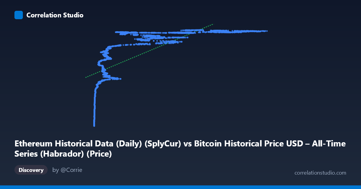
Ethereum Historical Data (Daily) (SplyCur) vs Bitcoin Historical Price USD – All-Time Series (Habrador) (Price)
- Pearson correlation (r)
- 0.6753
- Spearman correlation
- 0.9051
- p-value
- 0
- Sample size (n)
- 3926
- 95% confidence interval
- 0.6579 to 0.692
- Granger causality
- None
- Granger optimal lag
- 10
AI analysis
Analysis: Ethereum Supply (X) vs. Bitcoin Price (Y)
1. What the Visualization Reveals
Despite the column labels suggesting an "Ethereum vs. Bitcoin" price comparison, the actual data being correlated is Ethereum's circulating supply against Bitcoin's USD price — two time series that are both simply trending upward over the 2015–2026 window. The scatter shows a clear but curved relationship: Y rises steeply at low X values (under ~20,000 ETH-supply-units), then flattens into a plateau around 118–121 million as X continues climbing into the 60,000–125,000 range. This is a classic saturating/logarithmic curve shape, not a straight line, and it's really an artifact of two unrelated series both increasing over calendar time.
2. Strength, Direction, and Statistical Caveats
The Pearson correlation (r = 0.675, r² = 0.456) indicates a moderate positive linear relationship, with only 45.6% of Y's variance explained by X in a linear model — leaving over half unexplained. The tight confidence interval [0.658, 0.692] and p-value of ~0 confirm this correlation is statistically robust and not due to chance, given the large sample (n=3,926). However, statistical significance here reflects the large sample size and shared time trend, not necessarily a meaningful causal or economic linkage. Critically, the Granger causality tests show no predictive direction in either direction (X→Y: p=0.94; Y→X: p=0.82) — meaning past values of one series do not help forecast the other. This strongly suggests the correlation is spurious, driven by both variables independently trending over time rather than one influencing the other.
3. Notable Patterns and Non-linearity
The relationship is visibly non-linear: rapid growth in Y at low X, followed by a long flat plateau — consistent with logarithmic or asymptotic growth curves. The note that Spearman's ρ exceeds Pearson's r reinforces this: rank-order correlation is stronger than linear correlation, confirming a monotonic but curved relationship. A polynomial or log-transform of X (e.g., y = a·ln(x) + b) would likely fit dramatically better than the current linear model (R²=0.456). The clustering of points near the plateau (Y ≈ 119–121M) across a wide X range (20,000–125,000) is the dominant visual feature and drives most of the "explained" variance — the low-X, low-Y tail is doing the heavy lifting for the correlation coefficient.
4. Confounding Factors and Interpretation Caveats
The primary confound is time itself: both Ethereum's supply (which mechanically grows via block issuance) and Bitcoin's price (which has trended upward across market cycles) are monotonically related to calendar date. This is a textbook case of trend-driven spurious correlation — two unrelated non-stationary time series will almost always show significant correlation simply because both move directionally with time. The lack of Granger causality is the key diagnostic confirming this: if the relationship were substantive, we'd expect at least weak lead-lag predictability. Additionally, mixing a supply metric (ETH units in circulation) with a price metric (BTC USD) is a category mismatch — these aren't economically comparable quantities.
5. Recommendations for Further Investigation
- Detrend or difference both series (e.g., use daily/weekly returns or growth rates instead of levels) and re-run correlation — this is standard practice for non-stationary financial/time-series data and would likely collapse the correlation substantially. - Re-examine variable definitions: confirm whether "SplyCur" (Ethereum supply) was intended as the X-axis, or if a data-pipeline error swapped in supply where ETH price was meant — the column labels appear mismatched with the described dataset content. - Fit a log/polynomial model to quantify the non-linear relationship better, but interpret any improved R² cautiously given the causality findings. - Use cointegration tests (e.g., Engle-Granger) rather than simple correlation, which is the appropriate framework for assessing genuine long-run relationships between trending time series. - Treat this correlation as descriptive, not predictive or causal — it should not be used for forecasting one variable from the other.
X dataset: Bitcoin Historical Price USD – All-Time Series (Habrador)
Y dataset: Ethereum Historical Data (Daily)
Part of experiment: Bitcoin - Bitcoin Historical Price USD – All-Time Series (Habrador) vs Ethereum Historical Data (Daily)