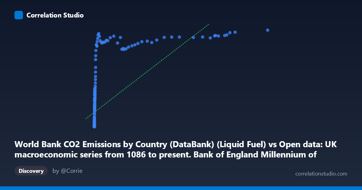
World Bank CO2 Emissions by Country (DataBank) (Liquid Fuel) vs Open data: UK macroeconomic series from 1086 to present. Bank of England Millennium of Macroeconomic Data. (Month) (value)
- Pearson correlation (r)
- 0.6597
- Spearman correlation
- 0.9578
- p-value
- 0
- Sample size (n)
- 267
- 95% confidence interval
- 0.5861 to 0.7226
- Granger causality
- Y → X
- Granger optimal lag
- 10
AI analysis
Analysis: UK Macroeconomic Activity vs. CO2 Liquid Fuel Emissions
1. Overall Relationship Pattern
The scatterplot reveals a broadly positive but clearly non-linear relationship between UK macroeconomic output (X-axis, liquid fuel CO2 emissions proxy) and CO2 emissions values (Y-axis). The data spans an extraordinary temporal range (1751–2017), capturing the full arc of industrialization, fossil fuel dependency, and potentially post-industrial decoupling. The most visually striking feature is a logarithmic or square-root-shaped curve: Y values rise steeply at low X values, then flatten dramatically at higher X values, creating a classic saturation pattern. This means that beyond a certain threshold of economic/emissions activity, additional increases in X produce diminishing returns in Y — consistent with an economy that has partially decoupled carbon intensity from output growth.
2. Correlation Strength, Direction, and Causality
The Pearson correlation of r = 0.66 (95% CI: [0.586, 0.723], p ≈ 0) confirms a statistically significant positive association, but the r² of 0.435 means the linear model explains only 43.5% of the variance in Y — leaving more than half unexplained by a straight-line fit. This is a meaningful limitation. Critically, the note that Spearman ρ exceeds Pearson r is important: it confirms the relationship is monotonic but non-linear, and a logarithmic or polynomial regression would almost certainly outperform the fitted linear equation (y = 0.161x + 2036.56). The Granger causality analysis adds a crucial temporal dimension: Y Granger-causes X (F = 2.376, p = 0.011) at a 10-period lag, but X does not Granger-cause Y (F = 1.486, p = 0.145). This unidirectional result suggests that CO2 emissions levels predictively precede macroeconomic changes — plausibly reflecting energy consumption as a leading indicator of industrial activity — rather than economic output driving emissions in a simple forward direction.
3. Notable Patterns, Clusters, and Outliers
Three distinct structural zones are visible in the data:
- Low-X cluster (X < ~500): A dense concentration of points near the origin, many with Y = 0.00, representing the pre-industrial or early-industrial era (pre-~1900) where liquid fuel emissions were negligible and macroeconomic values were correspondingly low or unrecorded. - Mid-range transition zone (X: 500–10,000): Points spread upward rapidly, consistent with the 20th-century industrialization and fossil fuel expansion period. - High-X plateau (X 10,000): Several extreme X-values (up to 116,836) with Y values that plateau around 11,000–13,600 — notably the point (116,836, 13,602) is a potential high-leverage outlier that likely exerts disproportionate influence on the linear regression coefficients. The Y-axis appears bounded near ~13,600, suggesting a data cap or natural ceiling.
4. Confounding Factors and Caveats
Several important caveats temper interpretation:
- Temporal confounding is severe: Both series trend upward over 266 years due to population growth, technological change, and measurement improvements — a classic spurious correlation from shared time trends. The correlation may largely reflect "both things grew over time" rather than a structural causal mechanism. - Dataset mismatch: X is labeled as World Bank CO2 Liquid Fuel data yet placed on the macroeconomic axis, while Y is described as a macroeconomic series but sourced from the CO2 dataset — the axis labels appear inverted or cross-joined, which warrants verification before drawing policy conclusions. - Aggregation issues: The N=18,769 population vs. n=267 sample suggests significant downsampling; monthly-to-annual alignment may introduce temporal mismatches. - Structural breaks: Events like WWI, WWII, the 1970s oil shocks, and post-2008 deindustrialization would create regime shifts invisible in aggregate correlation statistics.
5. Actionable Insights and Further Investigation
Recommended next steps:
1. Fit a logarithmic model (y = a·ln(x) + b) or power function — given the Spearman Pearson signal, this would likely raise explained variance well above 43.5% and yield more meaningful slope interpretation. 2. Detrend both series (first-differences or HP filter) to isolate cyclical co-movement and remove the spurious time-trend component before re-computing correlation and Granger tests. 3. Verify axis/dataset assignments — the apparent inversion of dataset descriptions between axes should be resolved to ensure causal interpretation is directionally correct. 4. Segment by historical era (pre-1900, 1900–1970, 1970–2017) to test whether the correlation structure changes across industrialization phases — the post-1970 period may show decoupling that is masked in the pooled analysis. 5. Investigate the 10-period Granger lag: At annual frequency, a 10-year lag for Y→X is economically interpretable as long-horizon energy infrastructure investment cycles; this deserves impulse-response analysis via a formal VAR model.
X dataset: Open data: UK macroeconomic series from 1086 to present. Bank of England Millennium of Macroeconomic Data. (Month)
Y dataset: World Bank CO2 Emissions by Country (DataBank)
Part of experiment: Yearly - Open data: UK macroeconomic series from 1086 to present. Bank of England Millennium of Macroeconomic Data. (Month) vs World Bank CO2 Emissions by Country (DataBank)