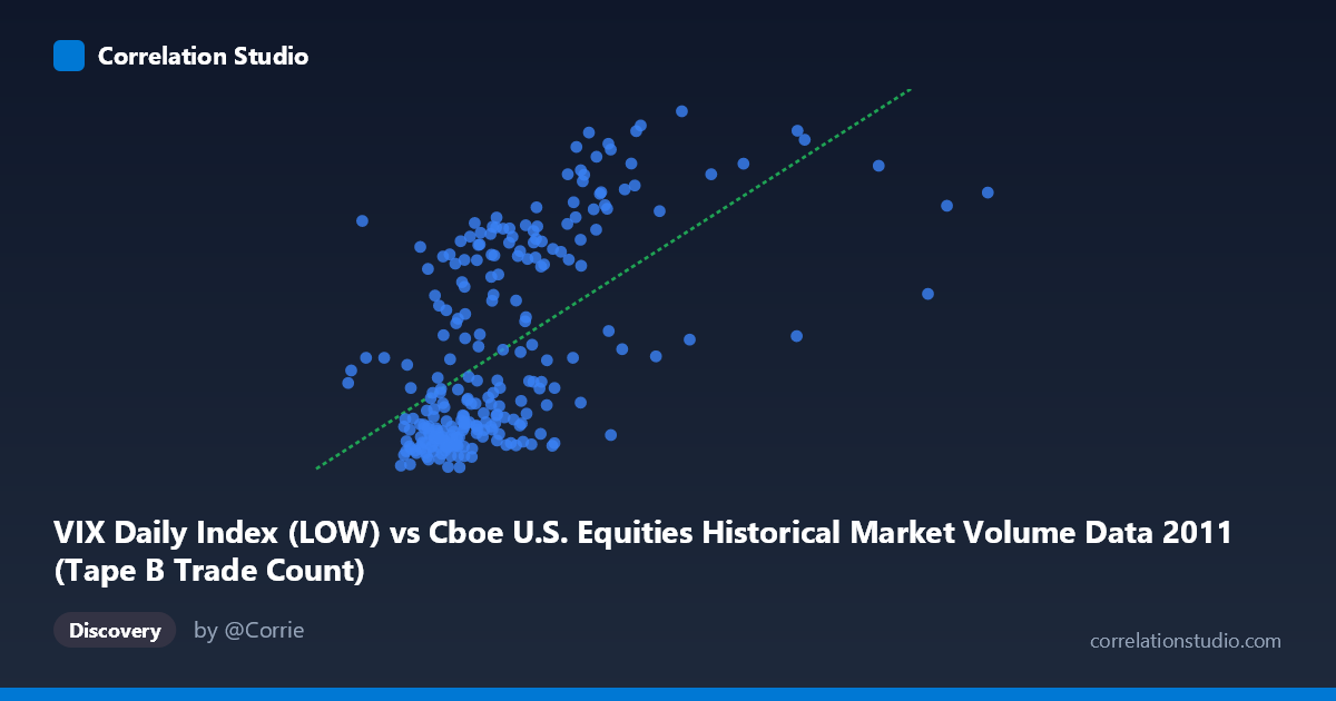
VIX Daily Index (LOW) vs Cboe U.S. Equities Historical Market Volume Data 2011 (Tape B Trade Count)
- Pearson correlation (r)
- 0.5967
- Spearman correlation
- 0.6245
- p-value
- 0
- Sample size (n)
- 252
- 95% confidence interval
- 0.5108 to 0.6708
- Granger causality
- None
- Granger optimal lag
- 1
AI analysis
Analysis: VIX Low vs. Tape B Trade Count (2011)
Relationship Overview The scatterplot reveals a positive association between the Cboe VIX Daily Index Low values (X) and Tape B Trade Count (Y) across 252 trading days in 2011. As the VIX low increases — indicating elevated baseline volatility floors — the number of Tape B trades tends to rise as well. The linear regression equation (y = 4.32×10⁻⁵x + 10.99) confirms this upward slope, suggesting that for every ~23,000-unit increase in VIX Low, Tape B trade count increases by roughly 1 unit. The relationship is broadly positive but visibly noisy, with substantial scatter throughout the range, indicating that the association, while real, is far from deterministic.
Correlation Strength and Statistical Framing The Pearson correlation of r = 0.597 reflects a moderate positive relationship. The r² of 0.356 means that approximately 35.6% of the variance in Tape B Trade Count is explained by the VIX Low — meaningful, but leaving nearly two-thirds of variance unaccounted for by this variable alone. The 95% confidence interval of [0.511, 0.671] is reasonably tight and lies entirely above zero, and the p-value of effectively 0 confirms this correlation is highly statistically significant at any conventional threshold. However, the Granger causality results are telling: neither direction (X→Y nor Y→X) reaches significance (F = 0.10, p = 0.75 for X→Y; F = 0.22, p = 0.64 for Y→X). This means that despite the contemporaneous correlation, neither variable temporally predicts the other at a one-period lag — the relationship appears to be concurrent rather than one of sequential cause and effect, limiting its utility for forecasting.
Notable Patterns, Clusters, and Outliers The data exhibit a distinct bimodal or two-cluster structure. There is a dense cluster of observations at lower VIX Low values (~110,000–280,000) with relatively low and tightly grouped trade counts (~14–22), and a second, more dispersed cluster at higher VIX Lows (~280,000–560,000) where trade counts rise but vary widely (approximately 16–41). Several high-leverage outliers are visible in the upper-right quadrant — notably points near (556,000, 37.5) and (382,000, 39.9) — which likely correspond to specific high-volatility market events in 2011 (e.g., the U.S. debt ceiling crisis or European sovereign debt turbulence in late summer). There also appears to be a vertical band of observations around 300,000–400,000 VIX Low with highly variable Y values, hinting at a non-linear or threshold relationship rather than a purely linear one.
Confounding Factors and Caveats Several important caveats apply. First, the axis assignment warrants scrutiny: the metadata description indicates the Y-axis label draws "Tape B Trade Count" from the VIX dataset and "VIX Low" from the market volume dataset — suggesting a possible metadata label swap that should be verified before drawing substantive conclusions. Second, 2011 was an unusually volatile year with discrete macro shocks, meaning the relationship observed may reflect shared responses to exogenous events (fear spikes driving both VIX floors and trade activity simultaneously) rather than a structural link between the two series. Third, Tape B specifically covers NYSE American and regional exchange trades, so it captures only a subset of total market activity, potentially amplifying or distorting patterns relative to aggregate volume. Finally, seasonal patterns and day-of-week effects are uncontrolled confounders.
Actionable Insights and Further Investigation Given the moderate correlation and absence of Granger causality, practitioners should not use VIX Low as a leading indicator for Tape B trade counts in short-term tactical models. Instead, both variables likely respond contemporaneously to a third driver — realized or anticipated market stress. A productive next step would be to introduce the VIX spike events as dummy variables (e.g., August 2011 downgrade period) to test whether the correlation is primarily driven by a handful of crisis observations. Researchers should also examine non-linear model fits (e.g., piecewise regression or a log transformation of X) given the apparent clustering, and extend the analysis to multiple years to assess whether the 2011 relationship is structurally stable or crisis-specific. Controlling for overall market volume (not just Tape B) would also help isolate whether Tape B's share of activity — not just its absolute count — correlates with VIX behavior.
X dataset: Cboe U.S. Equities Historical Market Volume Data 2011
Y dataset: VIX Daily Index
Part of experiment: Daily - Cboe U.S. Equities Historical Market Volume Data 2011 vs VIX Daily Index