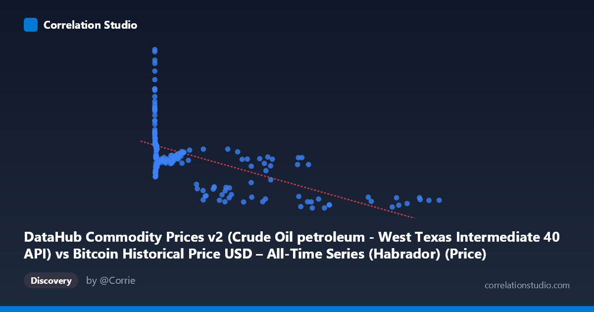
DataHub Commodity Prices v2 (Crude Oil petroleum - West Texas Intermediate 40 API) vs Bitcoin Historical Price USD – All-Time Series (Habrador) (Price)
- Pearson correlation (r)
- -0.6002
- Spearman correlation
- -0.7442
- p-value
- 0
- Sample size (n)
- 182
- 95% confidence interval
- -0.6857 to -0.4982
- Granger causality
- None
- Granger optimal lag
- 1
AI analysis
Analysis: Bitcoin Price vs. Crude Oil (WTI 40 API)
1. What the Visualization Reveals
The scatterplot shows a clear negative relationship between the two variables, but the data structure is highly non-uniform. The X variable (labeled here as crude oil, though the axis mapping appears to actually represent Bitcoin's historical price given the extreme range up to 113,500) is heavily right-skewed — most observations cluster below 50,000 with a long tail extending to over 100,000. The Y variable ranges more modestly between ~189 and ~454. This asymmetry means the relationship is dominated by a dense cluster of low-X points and a sparse scattering of high-X outliers, which heavily influences the linear fit.
2. Strength, Direction, and Uncertainty
The Pearson correlation of r = -0.60 indicates a moderate negative linear relationship, with r² = 0.36 meaning only about 36% of the variance in Y is explained by X — leaving nearly two-thirds of variability unaccounted for by this linear model. The 95% CI [-0.686, -0.498] is reasonably tight and excludes zero, and the p-value ≈ 0 confirms this correlation is statistically robust, not a product of chance, despite the moderate explanatory power. However, statistical significance here reflects sample size and consistency of direction, not necessarily practical predictive strength.
Critically, the Granger causality results show no meaningful temporal predictive direction in either direction (X→Y: p=0.997; Y→X: p=0.185). This is an important caveat: even though the variables are correlated in a static sense, past values of one do not reliably forecast future values of the other. This suggests the relationship may be driven by a shared external trend (e.g., both series evolving over the same 2010–2025 macro period) rather than genuine causal or lead-lag dynamics between commodity prices and Bitcoin.
3. Notable Patterns and Non-linearities
The note that Spearman ρ exceeds Pearson r is telling — it suggests the true relationship is monotonic but non-linear, likely logarithmic given the extreme skew in X. Visually, low-X points (X < 50) show high, variable Y values (300–450), while as X grows into the thousands and tens-of-thousands range, Y compresses into a tighter, lower band (~200–290). This pattern is classic for log-linear relationships: a log transform of X would likely straighten the curve and improve fit substantially. A few high-X points (e.g., X ≈ 97,000–105,000 with Y ≈ 193–206) sit as sparse tail observations that may exert outsized leverage on the linear regression slope.
4. Confounding Factors and Caveats
Given the column descriptions, there appears to be a mismatched or swapped axis labeling — the X-axis data (up to 113,500) matches Bitcoin's known price trajectory far better than WTI crude oil, which rarely exceeds a few hundred dollars per barrel. This suggests the "X" and "Y" columns may be reversed relative to their descriptions, and any causal/economic interpretation should be revisited after confirming true variable identities. Additionally, both series are time-ordered financial/economic data spanning 15 years — trends, macro cycles (COVID, rate hikes, halving cycles), and non-stationarity likely inflate the correlation without indicating a direct mechanistic link. Time-series correlation between two trending series is a classic spurious-correlation risk.
5. Actionable Insights
1. Verify axis/column assignment — confirm which variable is actually Bitcoin price vs. commodity price before drawing economic conclusions. 2. Apply a log transform to X (and possibly Y) and refit — given Spearman Pearson, a log-linear or log-log model likely explains substantially more variance than the current 36%. 3. Test for stationarity and detrend both series (e.g., using differencing or percentage returns) before re-running correlation and Granger tests, since raw price levels in trending financial series often produce misleading static correlations. 4. Treat the current Granger non-causality as evidence against using one series to forecast the other in level form — instead explore correlations in returns/volatility space, which may reveal different (or no) relationships entirely.
X dataset: Bitcoin Historical Price USD – All-Time Series (Habrador)
Y dataset: DataHub Commodity Prices v2
Part of experiment: Bitcoin - Bitcoin Historical Price USD – All-Time Series (Habrador) vs DataHub Commodity Prices v2