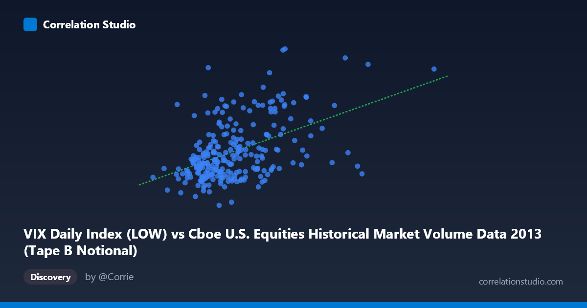
VIX Daily Index (LOW) vs Cboe U.S. Equities Historical Market Volume Data 2013 (Tape B Notional)
- Pearson correlation (r)
- 0.4701
- Spearman correlation
- 0.4304
- p-value
- 0
- Sample size (n)
- 252
- 95% confidence interval
- 0.3679 to 0.5611
- Granger causality
- None
- Granger optimal lag
- 1
AI analysis
Scatterplot Analysis: VIX Tape B Notional vs. Cboe Market Volume (VIX Low)
Overall Relationship The scatterplot reveals a moderate positive relationship between the VIX Daily Index Low values (X-axis, representing daily equity market volume metrics) and Tape B Notional values (Y-axis, representing VIX volatility index readings). As market volume figures increase, VIX readings tend to drift upward, suggesting that elevated trading activity in U.S. equities is associated with higher volatility readings. However, the scatter is substantial, and the relationship is far from deterministic — a wide band of Y values exists across nearly all ranges of X, indicating considerable noise in the association.
Correlation Strength and Statistical Significance The Pearson correlation of r = 0.4701 indicates a moderate positive association, but the explanatory power is limited: r² = 0.221 means only 22.1% of the variance in Tape B Notional is explained by the VIX Low values, leaving roughly 78% attributable to other factors. The 95% confidence interval [0.368, 0.561] is meaningfully above zero and does not include it, and the p-value of 2.89×10⁻¹⁵ confirms the correlation is highly statistically significant — effectively ruling out chance as an explanation given the sample of n = 252 from a population of N = 3,780. The linear regression equation (y = 6.75×10⁻¹⁰x + 11.18) reflects a very shallow positive slope, consistent with the modest but real trend. Critically, however, Granger causality tests in both directions are non-significant (X→Y: F = 1.03, p = 0.31; Y→X: F = 1.14, p = 0.29), meaning neither variable temporally predicts the other at a 1-period lag. This is an important caveat: the correlation is contemporaneous rather than directionally predictive, limiting its use for forecasting.
Notable Patterns, Clusters, and Outliers Several structural features are visible in the data. The bulk of observations cluster in the X range of approximately 2.5–5.0 billion, with Y values concentrated between 12 and 16, forming a relatively dense core. Beyond X ≈ 5.5 billion, the data becomes sparse, with a handful of notable high-volume outliers — particularly around X = 6.5–7.3 billion — that tend to pull the regression line. On the Y-axis, several high-VIX outliers are apparent near Y = 18–19 (e.g., the point at approximately X = 5.19B, Y = 18.98 and another near X = 4.66B, Y = 17.08), which sit well above the regression line and may correspond to specific market stress events during 2013. The distribution appears somewhat heteroscedastic, with Y variance appearing to widen at higher X values, which could violate linear regression assumptions.
Confounding Factors and Caveats Several important caveats apply. First, the axis labels appear inverted relative to intuition: VIX is plotted on the Y-axis while the market volume metric is on the X-axis, yet both datasets are labeled from each other's source files, suggesting a potential data mapping issue that warrants verification. Second, both variables are time-series from the same calendar year (2013), making serial autocorrelation a likely concern — observations are not independent, which can inflate apparent significance. Third, common external drivers such as macroeconomic announcements, Federal Reserve policy events (notably the 2013 "Taper Tantrum" in May–June), or earnings seasons could simultaneously drive both volume and volatility, creating a spurious correlation. Fourth, the non-significant Granger causality suggests the relationship is contemporaneous rather than causal, meaning both variables likely respond to the same underlying shocks rather than one causing the other.
Actionable Insights and Further Investigation Practitioners should treat this correlation as a contemporaneous market regime indicator rather than a predictive tool — high volume days and high VIX readings tend to co-occur, likely during risk-off or high-uncertainty market events. For further investigation, it would be valuable to: (1) decompose the time series to remove trend and seasonality before re-testing correlation, addressing autocorrelation concerns; (2) test at longer Granger lags (2–5 periods) to check whether predictive relationships emerge over slightly longer horizons; (3) identify and annotate the outlier dates (particularly the extreme Y values near 19) to determine whether they cluster around identifiable macro events like the Taper Tantrum; and (4) apply a non-linear model (e.g., polynomial or spline regression) given the potential heteroscedasticity and apparent non-linearity suggested by the scatter pattern. Segmenting data by market regime (low vs. high volatility periods) could also reveal whether the correlation strengthens meaningfully during stress periods.
X dataset: Cboe U.S. Equities Historical Market Volume Data 2013
Y dataset: VIX Daily Index
Part of experiment: Daily - Cboe U.S. Equities Historical Market Volume Data 2013 vs VIX Daily Index