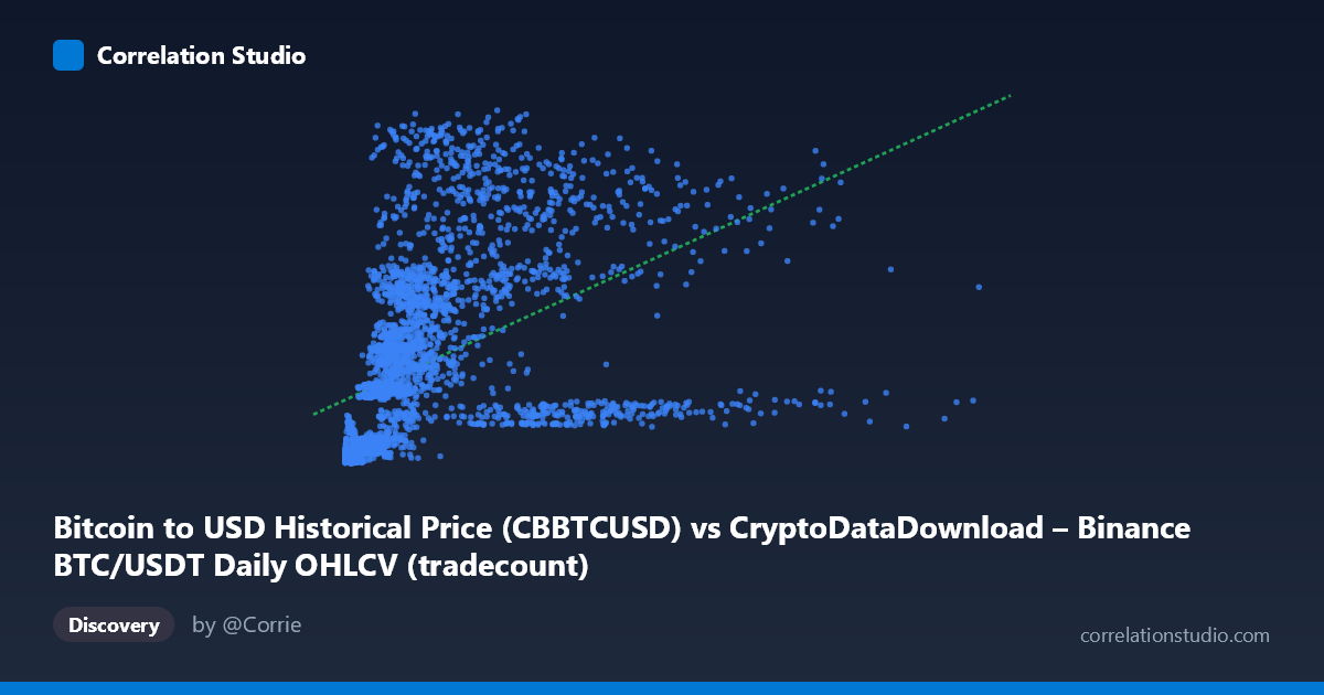
Bitcoin to USD Historical Price (CBBTCUSD) vs CryptoDataDownload – Binance BTC/USDT Daily OHLCV (tradecount)
- Pearson correlation (r)
- 0.4485
- Spearman correlation
- 0.7462
- p-value
- 0
- Sample size (n)
- 3211
- 95% confidence interval
- 0.4205 to 0.4758
- Granger causality
- None
- Granger optimal lag
- 10
AI analysis
Analysis: BTC/USDT Trading Volume vs. Trade Count (Binance)
1. What the Visualization Reveals
Despite the axis labels referencing "Bitcoin to USD Historical Price," the actual data being plotted is Binance BTC/USDT trading volume (X) against tradecount (Y) — the number of individual trades executed per day. The scatterplot shows a positive but noisy relationship: as daily volume increases, the number of trades tends to rise, but the relationship is far from deterministic. Points are widely scattered around any fitted line, especially at higher volume levels, indicating that volume alone is an incomplete predictor of trade count.
2. Strength, Direction, and Statistical Confidence
The correlation (r = 0.4485) is moderate and positive, but r² = 0.2012 means volume explains only about 20% of the variance in trade count — leaving 80% attributable to other factors (e.g., average trade size, market participant behavior, algorithmic vs. retail activity mix). The 95% CI [0.421, 0.476] is tight given the large sample (n=3,211), and the p-value of ~0 confirms this correlation is statistically robust and not due to chance — but statistical significance here reflects sample size more than practical strength.
The Granger causality tests are notable: neither direction shows significant predictive causality (X→Y: p=0.104; Y→X: p=0.847). This means past volume values do not reliably help forecast future tradecount (or vice versa) beyond what tradecount's own history provides. Practically, this suggests the relationship is contemporaneous/structural (both driven by common market activity) rather than one variable temporally leading the other — important for anyone trying to build a predictive trading signal from lagged volume or trade count.
3. Notable Patterns and Outliers
Several features stand out in the sampled data: - Heteroscedasticity: variance in tradecount increases with volume — low-volume days cluster tightly near low tradecounts (e.g., ~150K–900K volume with 3,500–12,000 trades), while high-volume days show much wider spread (e.g., ~$1M–5M volume producing anywhere from 20,000 to 123,000 trades). - Inconsistent scaling at high volume: some high-volume points (9.3M, 5.9M) correspond to relatively low tradecounts (~101K, ~20K), while moderate-volume points (2.7M, 2.5M) hit some of the highest tradecounts (~123K, ~116K) — suggesting average trade size varies substantially over time (possibly reflecting shifts between whale/institutional activity and high-frequency retail trading). - Non-linearity: the note that Spearman ρ exceeds Pearson r supports a curved (likely logarithmic or power-law) relationship — consistent with diminishing returns, where trade count grows sub-linearly as volume gets very large (large trades don't proportionally require more individual transactions).
4. Confounding Factors and Caveats
- Average trade size is the key latent variable: tradecount = volume / avg trade size, so shifts in market composition (bots vs. humans, institutional block trades vs. retail micro-orders) will decouple these two metrics independent of overall market activity. - Time-varying market regime: the 2017–2026 window spans multiple bull/bear cycles, exchange fee changes, and API/algorithmic trading growth — all of which could shift the volume-tradecount relationship non-stationarily over time, violating a naive pooled-correlation assumption. - Data labeling inconsistency: the metadata mismatch (price vs. volume/tradecount) raises concern about whether the underlying dataset is correctly aligned/joined — worth verifying before drawing strong conclusions.
5. Actionable Insights
- Fit a non-linear model (log-log or power-law regression) given the Spearman/Pearson divergence — this will likely improve explained variance meaningfully over the current 20%. - Segment by time period or market regime (e.g., bull vs. bear years) to check whether the volume-tradecount relationship is stable or structurally shifting — a regime-based or rolling-window correlation analysis would clarify this. - Investigate average trade size directly as a derived variable (volume/tradecount) to understand what's driving the scatter — this could reveal shifts in market microstructure (e.g., algo trading proliferation) that a raw scatterplot obscures. - Given the lack of Granger causality, don't use one variable to forecast the other in a trading strategy; treat both as joint indicators of market activity intensity rather than lead/lag signals.
X dataset: CryptoDataDownload – Binance BTC/USDT Daily OHLCV
Y dataset: Bitcoin to USD Historical Price
Part of experiment: Bitcoin - CryptoDataDownload – Binance BTC/USDT Daily OHLCV vs Bitcoin to USD Historical Price