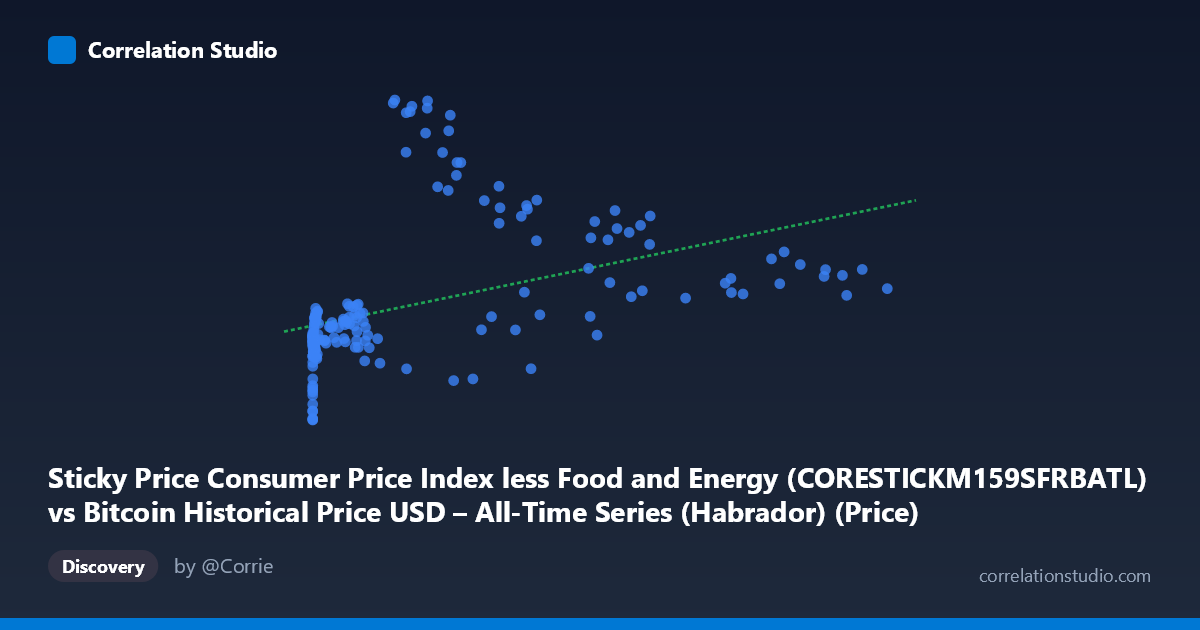
Sticky Price Consumer Price Index less Food and Energy (CORESTICKM159SFRBATL) vs Bitcoin Historical Price USD – All-Time Series (Habrador) (Price)
- Pearson correlation (r)
- 0.4314
- Spearman correlation
- 0.7276
- p-value
- 0
- Sample size (n)
- 189
- 95% confidence interval
- 0.3076 to 0.5408
- Granger causality
- None
- Granger optimal lag
- 1
- Time coverage
- 2010-08-01 to 2026-04-01
- Recomputed on refreshed data
- 2026-10-20 (r was 0.4314)
AI analysis
Analysis: Bitcoin Price vs. Sticky Price CPI (Core Inflation Index)
1. What the Visualization Reveals
The scatterplot shows a positive but noisy relationship between Bitcoin's historical USD price (X-axis) and the Sticky Price CPI less Food and Energy index (Y-axis, ranging 0.66–6.54). At very low Bitcoin prices (under $100, representing 2010-2013 data), the CPI values cluster tightly between 1.5–2.5. As Bitcoin prices climb into the tens of thousands, the Y values become more dispersed, ranging from ~1.6 to 6.5, with several high-value points (Y 4.5) appearing at X values above $20,000. This pattern is more consistent with a time-based coincidence than a direct causal or mechanical relationship — both series have simply trended upward over the 2010–2026 window.
2. Strength, Direction, and Statistical Confidence
The Pearson correlation of r = 0.431 indicates a moderate positive linear association, but r² = 0.186 means only about 18.6% of the variance in the CPI-related measure is explained by Bitcoin price (or vice versa) — leaving over 80% unexplained by this simple linear model. The 95% CI [0.308, 0.541] is reasonably tight and excludes zero, and the p-value (5.74×10⁻¹⁰) confirms the correlation is highly unlikely to be due to chance in this sample. However, statistical significance here reflects a real but weak association, not a strong predictive relationship. Critically, the Granger causality tests show no significant predictive direction in either direction (X→Y: p=0.758; Y→X: p=0.131) at lag 1. This strongly suggests the correlation is not driven by one variable temporally leading the other — it's more likely a spurious or third-factor-driven relationship, since both series are non-stationary trending time series (a classic setup for "spurious regression").
3. Notable Patterns and Non-linear Features
The data clearly shows a logarithmic/exponential curvature rather than a linear trend — Bitcoin's price spans nearly 7 orders of magnitude ($0.06 to $118,670), while Y only ranges from 0.66 to 6.54. Low-X points (X < 100) show consistently low, tightly clustered Y values (~1.5–2.5), while high-X points show much greater Y variance, including a notable cluster of high-Y outliers (5.0–6.5) at moderate-high X values (~19,000–30,000) alongside other high-X points with unremarkable Y values (~3.0–4.0) — indicating heteroscedasticity. The note that Spearman ρ exceeds Pearson r confirms a monotonic but non-linear relationship, meaning a log-transformed X variable would likely fit much better than the raw linear model (R²=0.186).
4. Confounding Factors and Caveats
The most significant caveat is that both variables are trending over the same 15+ year window (2010–2026) — Bitcoin price grew explosively while core CPI also rose steadily due to ordinary macroeconomic inflation. This shared time trend is a classic confound that inflates correlation between any two non-stationary series without implying causation. Additionally, comparing a monthly slow-moving inflation index to daily/volatile Bitcoin prices creates a scale/frequency mismatch, and the "N=701 vs n=189" gap suggests substantial subsampling or missing-data alignment issues that could bias results. The lack of Granger causality reinforces that this is very likely a spurious correlation via mutual time trend, not a genuine economic linkage.
5. Actionable Insights and Further Investigation
Rather than modeling raw levels, analysts should detrend both series (e.g., using year-over-year % changes or first differences) to test whether a genuine relationship persists once the shared time trend is removed — this is standard practice to avoid spurious regression in trending time series. A log-transform of Bitcoin price (given its exponential growth) should be tested against CPI, which may improve model fit per the Spearman signal. Given the null Granger causality result, it would also be worthwhile to test other macro variables (M2 money supply, real interest rates, dollar index) as potential joint drivers of both series, and to formally test both series for stationarity (e.g., ADF test) before drawing further causal or predictive conclusions.
X dataset: Bitcoin Historical Price USD – All-Time Series (Habrador)
Y dataset: Sticky Price Consumer Price Index less Food and Energy
Part of experiment: Bitcoin - Bitcoin Historical Price USD – All-Time Series (Habrador) vs Sticky Price Consumer Price Index less Food and Energy