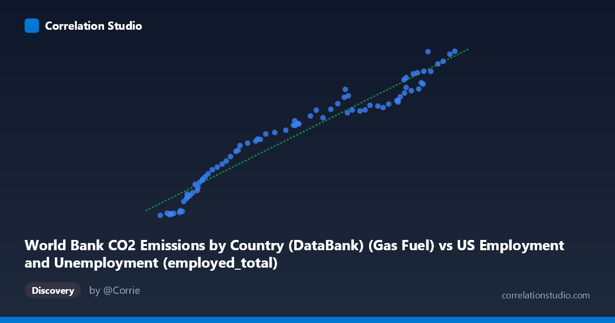
World Bank CO2 Emissions by Country (DataBank) (Gas Fuel) vs US Employment and Unemployment (employed_total)
- Pearson correlation (r)
- 0.9713
- Spearman correlation
- 0.9883
- p-value
- 0
- Sample size (n)
- 80
- 95% confidence interval
- 0.9554 to 0.9815
- Granger causality
- None
- Granger optimal lag
- 10
- Time coverage
- 1941-01-01 to 2020-01-01
AI analysis
Scatterplot Analysis: US Gas Fuel CO2 Emissions vs. Total US Employment (1941–2020)
Relationship Overview
The scatterplot reveals a striking positive linear relationship between US gas fuel CO2 emissions (X-axis) and total US employment (Y-axis) across eight decades of annual observations. As gas fuel emissions rise from roughly 50,000 to 157,000 units, total employment climbs from approximately 654,000 to nearly 17 million. The data points follow the regression line y = 0.137x − 5,051.25 with remarkable consistency, suggesting that both variables have been co-moving through time along a shared growth trajectory — almost certainly reflecting the long-run expansion of the US economy rather than any direct mechanistic link between emissions and job creation.
Correlation Strength and Statistical Interpretation
The Pearson correlation of r = 0.9713 is exceptionally strong, and the coefficient of determination R² = 0.9434 tells us that 94.3% of the variance in total employment is statistically explained by gas fuel CO2 emissions within this sample. The 95% confidence interval of [0.9554, 0.9815] is narrow and lies entirely in high-positive territory, confirming the estimate is precise and robust. The p-value of essentially zero rules out chance as an explanation for this association given N = 86 annual observations. However, the Granger causality tests complicate this picture considerably: neither direction (X→Y: F = 1.055, p = 0.414; Y→X: F = 0.720, p = 0.702) achieves statistical significance at any conventional threshold. This means that past values of emissions do not help predict future employment beyond what employment's own history provides, and vice versa — a critical finding that decouples the strong contemporaneous correlation from any claim of temporal predictive or causal direction.
Patterns, Clusters, and Notable Features
The data distribute into three loosely distinguishable regions that likely map onto historical periods. A dense lower-left cluster (X ≈ 50,000–70,000; Y ≈ 650–5,000) corresponds to earlier decades with lower economic activity and emissions. A middle band spanning X ≈ 70,000–120,000 shows some of the greatest scatter around the regression line, potentially reflecting periods of economic disruption (recessions, oil shocks) where the emissions-employment coupling loosened somewhat. The upper-right region (X 130,000; Y 11,000) is notably tight around the line. There are no dramatic outliers that would distort the regression, but a few points in the mid-range deviate noticeably, warranting investigation of which specific years they represent — candidates include recession years such as 1982, 2001, or 2008–2009.
Confounding Factors and Interpretive Caveats
The most significant caveat is spurious correlation driven by a shared time trend. Both US employment and CO2 emissions grew steadily over the 20th century as the US population expanded, the economy industrialized and then transitioned, and energy consumption scaled accordingly. This makes the high R² largely a reflection of two non-stationary time series moving together, not evidence of a substantive relationship. The Granger non-result reinforces this: when temporal structure is explicitly tested, predictive power disappears. Additional confounders include GDP growth, population size, and structural shifts in the energy mix (e.g., the natural gas boom post-2005 may have altered the emissions trajectory independently of employment). The dataset labeling also warrants scrutiny — the axis notes suggest a possible dataset-column mismatch (gas fuel emissions appearing in an employment dataset file, and vice versa), which could introduce data integrity concerns.
Actionable Insights and Further Investigation
Given the absence of Granger causality, analysts should detrend both series (e.g., using first differences or percentage changes) before drawing any policy-relevant conclusions — the residual correlation after detrending would be a far more meaningful signal. It would be valuable to test sector-specific employment (e.g., energy sector, manufacturing) against gas fuel emissions rather than total employment, as any genuine linkage would logically be concentrated there. Researchers should also model this relationship controlling for GDP and population to isolate whether emissions carry independent explanatory power. Finally, examining whether the relationship has structurally broken post-2010 — when US gas emissions and employment trends may have diverged due to renewable energy adoption and remote work patterns — could reveal important modern dynamics invisible in the aggregate 80-year view.
X dataset: US Employment and Unemployment
Y dataset: World Bank CO2 Emissions by Country (DataBank)
Part of experiment: Yearly - US Employment and Unemployment vs World Bank CO2 Emissions by Country (DataBank)