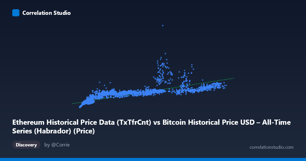
Ethereum Historical Price Data (TxTfrCnt) vs Bitcoin Historical Price USD – All-Time Series (Habrador) (Price)
- Pearson correlation (r)
- 0.8005
- Spearman correlation
- 0.948
- p-value
- 0
- Sample size (n)
- 3926
- 95% confidence interval
- 0.789 to 0.8115
- Granger causality
- None
- Granger optimal lag
- 10
AI analysis
Analysis: Ethereum Transfer Count vs. Bitcoin Price
1. Relationship Overview
The scatterplot shows a positive, moderately strong association between Ethereum's daily transaction transfer count (X) and Bitcoin's USD price (Y). As transfer counts rise from the low hundreds into the tens of thousands, Bitcoin price climbs from near-zero (early network history) into the hundreds of thousands to millions of dollars. However, the relationship is visibly non-linear: at low X values (under ~10,000 transfers), Y is compressed near the bottom of its range, while a small number of high-X points (75,000–125,000) correspond to some of the largest Y values, suggesting an accelerating or curved trend rather than a straight line.
2. Strength, Direction, and Statistical Confidence
The Pearson correlation of r = 0.80 indicates a strong positive linear relationship, with r² = 0.64 meaning roughly 64% of the variance in Bitcoin price is statistically associated with variance in Ethereum transfer counts — leaving over a third of the variance unexplained by this single variable. The 95% CI [0.789, 0.812] is tight, and the p-value is effectively 0, so we can be confident this correlation is not a sampling artifact given N≈3,926. However, statistical significance of correlation should not be conflated with causal predictive power: the Granger causality tests show no significant lead-lag relationship in either direction (X→Y p=0.84; Y→X p=0.86). This means neither series helps forecast the other's future values beyond its own history — the correlation is likely driven by both series sharing a common underlying trend (e.g., overall crypto market growth/adoption over time) rather than one variable mechanically driving the other.
3. Notable Patterns and Non-linearity
The data is heavily right-skewed in X (mean 30,451 vs. median likely much lower, stdev 32,538) and even more skewed in Y (mean 670,859, stdev 484,043, max 5.25 million) — the huge Y range and stdev relative to mean suggest extreme outliers or a late-stage price spike dominating the tail. The note that Spearman ρ exceeds Pearson r is important: it confirms the relationship is monotonic but not well-captured by a straight line — a logarithmic or power-law fit (common in crypto/network-value relationships, akin to Metcalfe's Law) would likely fit better than the linear model (y = 11.9x + 308,233). Visually, expect clustering of many points in the lower-left (small X, small-to-moderate Y) with a sparser, fanned-out upper-right tail where variance in Y increases dramatically for similar X values — classic heteroscedasticity.
4. Confounding Factors and Caveats
This comparison conflates two different assets' metrics (Ethereum activity vs. Bitcoin price) across an 11-year span (2015–2026), during which both underwent massive structural changes: exchange listings, halving cycles, regulatory shifts, DeFi/NFT booms, and macro liquidity cycles. The dominant confound is time itself — both series trend upward over the sample period, so the correlation may largely reflect shared secular growth (a spurious correlation pattern) rather than any direct economic link between ETH network usage and BTC valuation. Additionally, mismatched column labeling in the dataset (X labeled as Ethereum TxTfrCnt from a "Bitcoin" dataset, Y labeled as Bitcoin Price from an "Ethereum" dataset) raises data-hygiene concerns that should be verified before drawing conclusions.
5. Suggested Next Steps
1. Detrend or difference both series (e.g., % daily/monthly change) and re-run correlation and Granger tests to control for the shared time trend — this is critical given the null Granger result. 2. Fit log-log or power-law models given the Spearman/Pearson divergence and Metcalfe's-Law-like network effects common in crypto data. 3. Segment by market regime (bull vs. bear cycles) to check if correlation strength is stable or regime-dependent. 4. Verify column/dataset labeling to ensure X and Y are correctly sourced before publishing conclusions. 5. Treat this as a descriptive association, not a trading or forecasting signal, given the absence of Granger causality in either direction.
X dataset: Bitcoin Historical Price USD – All-Time Series (Habrador)
Y dataset: Ethereum Historical Price Data
Part of experiment: Bitcoin - Bitcoin Historical Price USD – All-Time Series (Habrador) vs Ethereum Historical Price Data