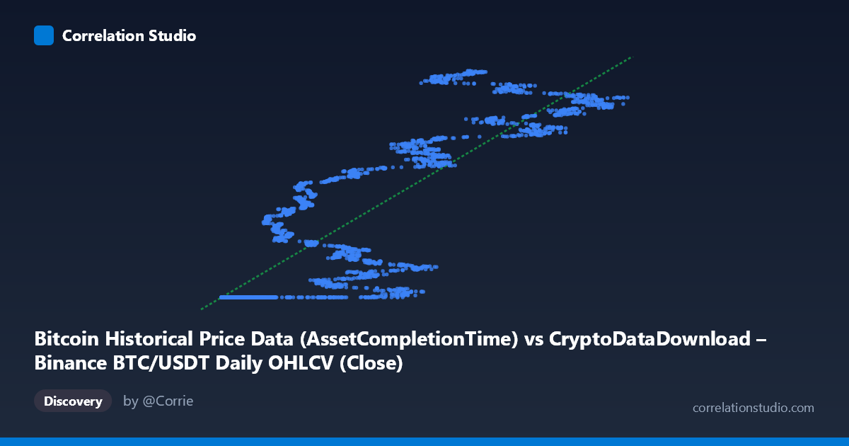
Bitcoin Historical Price Data (AssetCompletionTime) vs CryptoDataDownload – Binance BTC/USDT Daily OHLCV (Close)

Pearson correlation (r): 0.8518
Spearman correlation: 0.8876
p-value: 0
Sample size (n): 3191
95% confidence interval: 0.842 to 0.861
Granger causality: None
Granger optimal lag: 10
Time coverage: 2017-08-17 to 2026-05-20

AI analysis

Analysis of Bitcoin Price/Metric Relationship

1. Overview of the Relationship

This scatterplot compares "AssetCompletionTime" (X) against Bitcoin's Close price (Y), showing a positive, moderately strong association. As X increases, Y generally trends upward, though the relationship appears non-linear — with a distinct plateau/floor around Y≈1,614,337,000 for a wide range of low X values (roughly 3,000–25,000), followed by a steeper, more variable climb at higher X values. This suggests the relationship may be threshold-based or piecewise rather than strictly linear.

2. Strength, Direction, and Statistical Confidence

The correlation coefficient (r = 0.852) indicates a strong positive linear relationship, with r² = 0.726 meaning approximately 72.6% of the variance in Y is statistically explained by X — a substantial but incomplete share, leaving ~27% attributable to other factors or noise. The tight 95% CI [0.842, 0.861] and p-value of 0 (effectively p < 0.0001) confirm this correlation is highly statistically robust and not a product of sampling chance, especially given the large sample size (n=3,191). However, statistical significance and correlation strength say nothing about causality. The Granger causality tests reinforce this caution: neither direction (X→Y: p=0.326; Y→X: p=0.168) shows significant predictive causality at the tested lag (10 periods). This means past values of X do not meaningfully help forecast future Y (or vice versa) — the strong contemporaneous correlation likely reflects a shared underlying driver (e.g., calendar time itself, since X is literally a timestamp/completion-time field) rather than one variable dynamically predicting the other.

3. Notable Patterns and Anomalies

The most striking feature is the flat cluster at the low end of X (X < ~25,000), where Y is pinned near its minimum (~1,614,337,100) with almost no variance — this looks like a data floor, censoring artifact, or an early period where the price metric was constant/placeholder. Above this threshold, Y becomes highly dynamic, swinging between ~1.61B and ~1.78B with considerable scatter, indicating heteroskedasticity (non-constant variance) — a violation of standard linear regression assumptions. There also appear to be two loose "bands" in the higher-X region (e.g., values near 1.74B vs. 1.76–1.78B), hinting at possible sub-clusters or regime shifts rather than one smooth trend.

4. Caveats and Confounding Factors

Given that X is drawn from a "Historical Price Data (AssetCompletionTime)" column and Y is Bitcoin's Close price from the same underlying dataset lineage, it's likely both variables are proxies for time or are mechanically linked (e.g., X may encode a timestamp-derived value correlated with dataset progression rather than an independent economic driver). This raises serious concern about spurious correlation via a common time trend — both series may simply be trending together because Bitcoin price rose over the 2017–2026 window, not because X causally influences Y in any meaningful sense. The flat segment at low X further suggests a data quality issue (truncation, missing data backfilled with a constant, or an onboarding/initialization period) that should be scrutinized before drawing conclusions.

5. Recommendations for Further Investigation

1. Clarify variable definitions: Confirm what "AssetCompletionTime" actually represents — if it's a timestamp or index, the analysis should control for date/time explicitly (e.g., detrend both series) to test for spurious correlation. 2. Segment the analysis: Run separate regressions/correlations on the flat low-X cluster versus the dynamic high-X region, since pooling them likely inflates apparent linear fit while masking regime differences. 3. Investigate the plateau: Determine why Y is constant for X < 25,000 — check for data entry errors, placeholder values, or a genuine early-period phenomenon. 4. Test alternative functional forms: Given evident heteroskedasticity and possible piecewise structure, consider log-transformations, spline/piecewise regression, or quantile regression instead of simple OLS. 5. Treat the relationship as associative, not causal: Given the null Granger causality results, avoid using X to forecast Y (or vice versa) in any predictive model without further evidence of a genuine lead-lag mechanism.

X dataset: CryptoDataDownload – Binance BTC/USDT Daily OHLCV

Y dataset: Bitcoin Historical Price Data

Part of experiment: Bitcoin - CryptoDataDownload – Binance BTC/USDT Daily OHLCV vs Bitcoin Historical Price Data