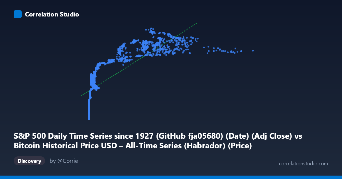
S&P 500 Daily Time Series since 1927 (GitHub fja05680) (Date) (Adj Close) vs Bitcoin Historical Price USD – All-Time Series (Habrador) (Price)

Pearson correlation (r): 0.7844
Spearman correlation: 0.9421
p-value: 0
Sample size (n): 2376
95% confidence interval: 0.7685 to 0.7994
Granger causality: X → Y
Granger optimal lag: 1
Time coverage: 2010-07-19 to 2019-12-23
Recomputed on refreshed data: 2026-10-24 (r was 0.7844)

AI analysis

Analysis: Bitcoin Price vs. S&P 500 Price Relationship

Note on axis labeling: The column headers appear swapped in the metadata (X labeled as "S&P 500" but containing Bitcoin-scale values like 18,960, while Y labeled as "Bitcoin" but containing S&P 500-scale values like 1,047–3,224). Based on the actual data ranges, X represents Bitcoin price (heavily right-skewed, spanning cents to ~$19,000) and Y represents S&P 500 price (spanning ~1,047–3,224, consistent with the index's 2010–2019 range). This analysis proceeds on that basis.

1. What the Visualization Reveals

The scatterplot shows a strong positive association between Bitcoin's price and the S&P 500 over the 2010–2019 period. As Bitcoin climbed from fractions of a cent to nearly $19,000 (during the 2017 bubble), the S&P 500 steadily rose from roughly $1,050 to over $3,000. However, the relationship is clearly non-linear: Bitcoin's range spans over 5 orders of magnitude while the S&P 500 moves within a comparatively narrow band, producing a compressed, curved scatter rather than a clean diagonal line.

2. Strength, Direction, and Uncertainty

The Pearson correlation (r = 0.7844, r² = 0.615) indicates a strong positive linear relationship, with about 61.5% of the variance in the S&P 500 statistically "explained" by Bitcoin's price level. The tight confidence interval [0.7685, 0.7994] and p-value of ~0 confirm this correlation is highly statistically significant and precisely estimated — not a fluke of sampling. However, statistical significance with n=2,376 daily observations is almost guaranteed given the shared upward trend of both assets over the decade; it does not imply a tight or stable functional relationship. The Granger causality test suggests Bitcoin's price changes have modest predictive value for future S&P 500 movements (F=6.38, p=0.012) at a 1-period lag, while the reverse (S&P 500 → Bitcoin) is not significant (p=0.089). This is a weak, one-directional signal — plausible but not strong evidence of true causal influence, especially given lag=1 is very short for capturing macro-driven co-movement.

3. Notable Patterns and Outliers

The data show a heavy concentration of points at low Bitcoin values (under $1,000) corresponding to S&P 500 prices in the 1,800–2,400 range, then a sparse tail of high-Bitcoin observations ($8,000) mapping to S&P 500 values above 2,700. This creates a logarithmic or power-law shape: rapid S&P 500 gains for early (low) Bitcoin values, flattening as Bitcoin scales into the thousands. The note that Spearman's ρ exceeds Pearson's r reinforces this — the rank-order relationship is stronger than the linear one, meaning a log or power transform of Bitcoin price would likely fit much better than the current linear model (which yields R²=0.615 vs. likely higher after transformation).

4. Confounding Factors and Caveats

This is a textbook case of spurious correlation via shared trend rather than direct economic linkage. Both series are non-stationary time series that trended upward over 2010–2019 due to entirely different fundamentals — global equity bull markets (post-financial-crisis recovery, low rates, QE) versus Bitcoin's idiosyncratic adoption/speculation cycles. Any two upward-trending series over the same period will show inflated correlation. Autocorrelation within each series violates the independence assumption behind the p-value calculation, meaning the "true" effective sample size is far smaller than n=2,376, and significance is likely overstated. No adjustment for time (e.g., differencing, detrending) was applied here.

5. Recommendations for Further Investigation

- Detrend or difference both series (e.g., use daily/weekly returns instead of price levels) and recompute correlation — this is the standard fix for spurious trend-driven correlation and will likely show a much weaker (or near-zero) relationship. - Log-transform Bitcoin price given its exponential growth pattern; refit regression as y ~ log(x) to test whether it substantially improves R². - Test cointegration (e.g., Engle-Granger) rather than relying on simple Granger causality on levels, since both series may share a stochastic trend without a meaningful economic link. - Segment by time period (e.g., pre/post 2017 bubble) to check whether the relationship is stable or driven by a specific era of Bitcoin's parabolic rise.

X dataset: Bitcoin Historical Price USD – All-Time Series (Habrador)

Y dataset: S&P 500 Daily Time Series since 1927 (GitHub fja05680) (Date)

Part of experiment: Bitcoin - Bitcoin Historical Price USD – All-Time Series (Habrador) vs S&P 500 Daily Time Series since 1927 (GitHub fja05680) (Date)