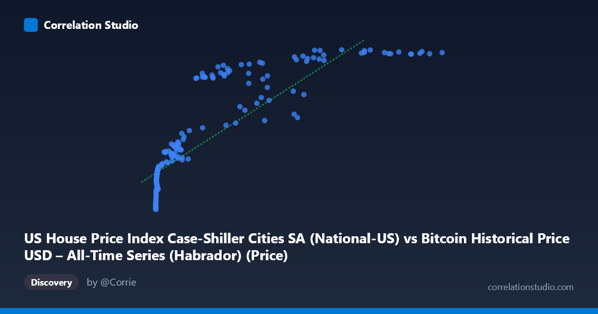
US House Price Index Case-Shiller Cities SA (National-US) vs Bitcoin Historical Price USD – All-Time Series (Habrador) (Price)
- Pearson correlation (r)
- 0.8512
- Spearman correlation
- 0.9698
- p-value
- 0
- Sample size (n)
- 189
- 95% confidence interval
- 0.8065 to 0.8863
- Granger causality
- None
- Granger optimal lag
- 9
- Time coverage
- 2010-08-01 to 2026-04-01
- Recomputed on refreshed data
- 2026-10-22 (r was 0.847)
AI analysis
Analysis: Bitcoin Price vs. US House Price Index (Case-Shiller)
1. Relationship Overview
The scatterplot shows a strong positive association between Bitcoin's historical price (X-axis, spanning an extreme range from $0.06 to $118,670) and the Case-Shiller US House Price Index (Y-axis, ranging 136.5–332.1). The relationship is clearly non-linear: at low Bitcoin prices (under ~$1,000), the HPI values cluster tightly in the 137–190 range with very little spread, while as Bitcoin prices climb into the tens of thousands, HPI values rise more steeply and then begin to plateau/saturate near 320–330. This produces a curve reminiscent of a logarithmic or power-law shape rather than a straight line — consistent with the note that Spearman's ρ exceeds Pearson's r.
2. Strength, Direction, and Statistical Confidence
The Pearson correlation (r = 0.847) indicates a strong positive linear relationship, with r² = 0.717 meaning the linear model explains about 72% of the variance in HPI from Bitcoin price. The 95% CI [0.801, 0.883] is fairly tight and the p-value ≈ 0 confirms this correlation is highly unlikely due to chance, given n = 187. However, correlation strength should not be conflated with causation or predictive power over time: the Granger causality tests show no significant temporal predictive direction in either direction (Bitcoin→HPI: p=0.30; HPI→Bitcoin: p=0.12). This means neither series' past values meaningfully help forecast the other's future values at a 1-period lag — the strong contemporaneous correlation likely reflects both variables trending upward over the same historical period (2010–2026) rather than one driving the other.
3. Notable Patterns and Outliers
Several features stand out: - Compression at low X: Dozens of points with Bitcoin prices under $1,000 (even fractions of a cent) are compressed near HPI 137–190, reflecting Bitcoin's early years (2010–2013) when house prices were still near post-2008-crash lows. - Ceiling effect at high X: Once Bitcoin exceeds ~$60,000, HPI values saturate around 320–330, suggesting the housing index growth has slowed/plateaued while Bitcoin continued to swing wildly (e.g., $118,670 vs. $57,454 both correspond to HPI ~328–332). - Inversions/non-monotonic segments: Notably, (45092.81, 245.43) and (56973.18, 281.53) and (58724.66, 249.01) sit well below the trend of neighboring points with similar or lower X values (e.g., 41869.55→266.61, 34855.64→262.56), indicating Bitcoin crash periods (bear markets) where BTC price dropped temporarily while HPI kept climbing — clear evidence the two series periodically decouple. - These deviations reinforce that a single linear fit misses cyclical Bitcoin volatility that has no counterpart in the smoother, slower-moving HPI.
4. Confounding Factors and Caveats
This is a classic case of spurious correlation via shared time trend. Both Bitcoin price and US house prices have risen substantially from 2010 to 2026 due to largely unrelated macro forces — Bitcoin driven by adoption/speculation cycles, housing driven by low interest rates, post-2008 recovery, pandemic-era demand shifts, and constrained supply. Any two upward-trending time series over the same long window will show high correlation without genuine economic linkage. Additional caveats: extreme scale mismatch (X spans 6 orders of magnitude) means log-transforming X is likely necessary for meaningful linear modeling; the "n=187 of N=470" subsampling could introduce selection bias; and monthly HPI data being merged with volatile daily/irregular Bitcoin prices introduces alignment/aggregation artifacts.
5. Suggestions for Further Investigation
1. Re-fit using log(X) or polynomial regression — given the Spearman/Pearson gap, a log-linear or power model will likely explain substantially more variance and better represent the true shape. 2. Detrend both series (e.g., using year-over-year % change or differencing) before computing correlation, to test whether the relationship holds beyond mutual upward drift. 3. Run Granger causality on detrended/stationary series — the current non-significant result may partly reflect non-stationarity in both series masking true short-term lead-lag effects. 4. Treat this correlation as descriptive/historical co-movement, not a basis for using one asset to forecast the other; frame it as two independent bull markets coinciding in the 2010s–2020s rather than a causal economic linkage.
X dataset: Bitcoin Historical Price USD – All-Time Series (Habrador)
Y dataset: US House Price Index Case-Shiller Cities SA
Part of experiment: Bitcoin - Bitcoin Historical Price USD – All-Time Series (Habrador) vs US House Price Index Case-Shiller Cities SA