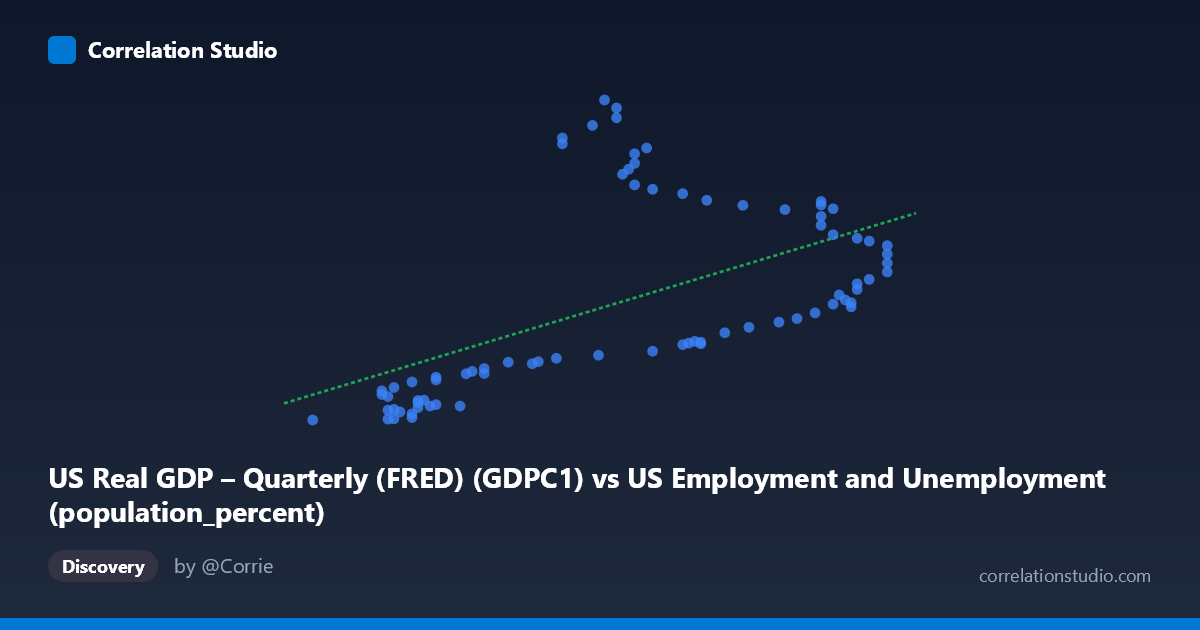
US Real GDP – Quarterly (FRED) (GDPC1) vs US Employment and Unemployment (population_percent)
- Pearson correlation (r)
- 0.5613
- Spearman correlation
- 0.6527
- p-value
- 0
- Sample size (n)
- 79
- 95% confidence interval
- 0.3884 to 0.696
- Granger causality
- None
- Granger optimal lag
- 10
- Time coverage
- 1947-01-01 to 2025-01-01
- Recomputed on refreshed data
- 2026-10-09 (r was 0.5618)
AI analysis
Analysis: US Real GDP vs. Employment-to-Population Percent
1. Overall Relationship
The scatterplot reveals a positive relationship between US Real GDP (x-axis, measured in billions of chained 2017 dollars) and the employment-to-population percentage (y-axis), spanning data from 1947 to 2025. As real GDP rises, the share of the population employed tends to increase alongside it, which is intuitively consistent with the idea that economic expansion generates jobs and draws more workers into the labor force. However, the scatter is notably wide, suggesting that GDP alone is far from a complete explanation of employment participation rates across this 78-year span.
2. Correlation Strength, Direction, and Causality
The correlation coefficient of r = 0.5618 indicates a moderate positive association. Critically, the R² of 0.3156 means that only ~31.6% of the variance in employment-to-population percentage is explained by real GDP, leaving nearly 70% attributable to other factors. The 95% confidence interval for r of [0.3890, 0.6964] is relatively wide, reflecting meaningful uncertainty in the true population relationship despite the highly significant p-value of 7.19×10⁻⁸, which confirms the association is extremely unlikely to be due to chance. The linear regression equation (y = 1214.56x − 66,021.9) implies each unit increase in GDP associates with roughly 1,215 additional percentage points of employment participation in scaled terms — but this should be interpreted cautiously given the moderate fit. Most importantly, the Granger causality tests find no significant predictive directionality in either direction (X→Y: F=1.42, p=0.20; Y→X: F=1.05, p=0.42), meaning that neither variable reliably predicts the other's future values even at an optimal lag of 10 periods. This substantially weakens any causal narrative and suggests the correlation may reflect shared trends rather than a direct mechanistic link.
3. Notable Patterns, Clusters, and Outliers
The data visibly clusters into two broad regimes rather than forming a clean linear cloud. At lower GDP values (roughly 57.5–61), employment percentages are tightly bunched between approximately 2,200 and 6,000 — a relatively compressed range. But in the mid-to-upper GDP range (62–67), the Y-values fan out dramatically, ranging from ~6,500 to over 23,500, creating a pronounced heteroscedastic pattern where variance in Y increases substantially with X. Several points stand out as potential outliers: values like (62.20, 21,932), (62.40, 23,548), (62.60, 23,082), and (61.70, 20,709 and 21,082) all show very high employment percentages at only moderate GDP levels, pulling strongly against the linear trend. This funnel-shaped dispersion is a strong visual signal that a simple linear model is inadequate and that important non-linear dynamics or structural breaks are present in the data.
4. Confounding Factors and Caveats
Several important confounds complicate interpretation. Secular demographic trends — including the baby boom, rising female labor force participation through the 1960s–1990s, and aging population dynamics post-2000 — directly affect employment-to-population ratios independent of GDP cycles. Structural economic shifts (manufacturing decline, service sector growth, gig economy emergence) alter the relationship between output and headcounts over time. The dataset spans 78 years across multiple distinct economic eras, meaning the relationship observed in 1947 is likely structurally different from that in 2025 — pooling them risks misleading inference. The lack of Granger causality also warns against assuming that GDP growth leads employment gains in any reliable temporal sense, which may reflect the well-known complexity of labor market adjustment lags and policy interventions (e.g., fiscal stimulus, unemployment insurance). Finally, the x-axis label appears to conflate two different datasets (GDP values are noted in what look like per-capita or ratio units near 57–67, which is unusual for GDPC1 in billions), suggesting possible data transformation or normalization issues that should be verified.
5. Actionable Insights and Further Investigation
Given the heteroscedasticity and clustering observed, non-linear or regime-switching models (e.g., polynomial regression, piecewise linear, or Markov-switching models) should be explored to better capture the true relationship. Researchers should consider segmenting the analysis by economic era (pre-1980, 1980–2008, post-2008) to test whether the correlation is stable or structurally shifting over time. Including additional control variables — such as labor force participation rate, demographic composition, inflation, and interest rates — in a multivariate framework would likely dramatically improve explained variance beyond the current 31.6%. The high-employment/moderate-GDP outlier cluster (around X=62–62.5, Y20,000) deserves specific investigation, as these data points may represent a particular historical period or measurement anomaly. Finally, verifying the units and transformations applied to both axes is essential before drawing any policy conclusions, as the unusually narrow GDP range (57–67) suggests these may be transformed or indexed values rather than raw GDPC1 billions.
X dataset: US Employment and Unemployment
Y dataset: US Real GDP – Quarterly (FRED)
Part of experiment: Yearly - US Employment and Unemployment vs US Real GDP – Quarterly (FRED)