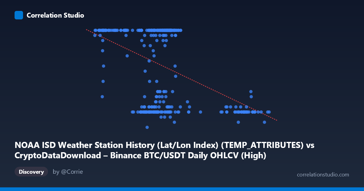
NOAA ISD Weather Station History (Lat/Lon Index) (TEMP_ATTRIBUTES) vs CryptoDataDownload – Binance BTC/USDT Daily OHLCV (High)
- Pearson correlation (r)
- -0.4675
- Spearman correlation
- -0.2951
- p-value
- 0
- Sample size (n)
- 355
- 95% confidence interval
- -0.5451 to -0.382
- Granger causality
- None
- Granger optimal lag
- 1
- Time coverage
- 2024-01-01 to 2024-12-31
AI analysis
Analysis of Variable Relationship
Note on labeling: The axis metadata appears mismatched/scrambled (X labeled as a weather station index but showing values like 40,000–108,000; Y labeled as BTC "High" price but ranging 5–24). Given the actual data, X behaves like a BTC price-related variable (~40k–108k) and Y behaves like a bounded count or index (5–24, likely temperature-like or a categorical/discrete score). I'll analyze the statistical relationship as presented, treating X and Y at face value from the numeric data.
1. Overall Relationship
The scatterplot shows a moderate negative linear relationship between X and Y. As X increases, Y tends to decrease, though the relationship is far from deterministic. The regression line (y = -0.000238x + 32.93) confirms this downward slope. Notably, Y is heavily concentrated at its ceiling value of 24 across a wide swath of X values (roughly 41,000–74,000), suggesting a possible censoring or saturation effect rather than a purely continuous linear relationship.
2. Strength, Direction, and Statistical Confidence
The correlation coefficient r = -0.4675 indicates a moderate negative association. However, r² = 0.2185 means only about 21.9% of the variance in Y is explained by X — the majority (78%) of Y's variability is driven by other factors. The 95% confidence interval [-0.5451, -0.3820] is reasonably tight and excludes zero, and the p-value ≈ 0 confirms this correlation is statistically significant and not due to chance, despite its modest explanatory power.
Critically, the Granger causality tests show no significant predictive direction in either direction (X→Y: p=0.708; Y→X: p=0.233). This means neither variable's past values help forecast the other's future values in a time-series sense. The correlation is likely contemporaneous/structural rather than causal or sequential — an important distinction, especially given the mismatched dataset labeling.
3. Notable Patterns and Outliers
Several distinct patterns emerge: - A dense cluster at Y=24 spanning X ≈ 41,000–74,000, suggesting a ceiling effect or a discrete category "maxing out" frequently in this X range. - A lower cluster (Y ≈ 7–12) appearing at both moderate X values (~60,000–75,000) and high X values (~91,000–101,000), indicating this isn't purely linear — there seem to be two behavioral regimes rather than one smooth trend. - High-X outliers (X 90,000) consistently show low Y values (8–11), pulling the regression slope negative and suggesting the relationship may be driven disproportionately by this sparse upper-X segment.
4. Confounding Factors and Caveats
- Metadata mismatch: The column descriptions don't align with the data ranges shown, raising concerns about data provenance/joining errors. This should be resolved before drawing domain conclusions. - Ceiling/censoring effect: Y's frequent value of exactly 24 suggests it may be capped, which violates assumptions of simple linear correlation and inflates or biases r². - Non-linearity: The apparent bimodal clustering suggests a linear model may be inadequate — a threshold or regime-based model might fit better. - Time-series structure ignored: Since this spans a full year (2024) of daily data, autocorrelation within each series (especially financial data) could inflate apparent correlation despite no Granger causality.
5. Recommended Next Steps
1. Verify data alignment — confirm the X/Y columns are correctly mapped to their intended sources before further interpretation. 2. Investigate the ceiling effect on Y=24 — determine if this reflects a true data cap, missing data imputation, or a genuine saturation phenomenon. 3. Test non-linear/segmented models (e.g., piecewise regression or clustering) given the visual bimodality. 4. Explore additional covariates that might explain the 78% unexplained variance, especially around the high-X, low-Y outlier cluster. 5. Given the lack of Granger causality, avoid using either variable to forecast the other; treat the relationship as associative only.
X dataset: CryptoDataDownload – Binance BTC/USDT Daily OHLCV
Y dataset: NOAA ISD Weather Station History (Lat/Lon Index)
Part of experiment: Bitcoin - CryptoDataDownload – Binance BTC/USDT Daily OHLCV vs NOAA ISD Weather Station History (Lat/Lon Index)