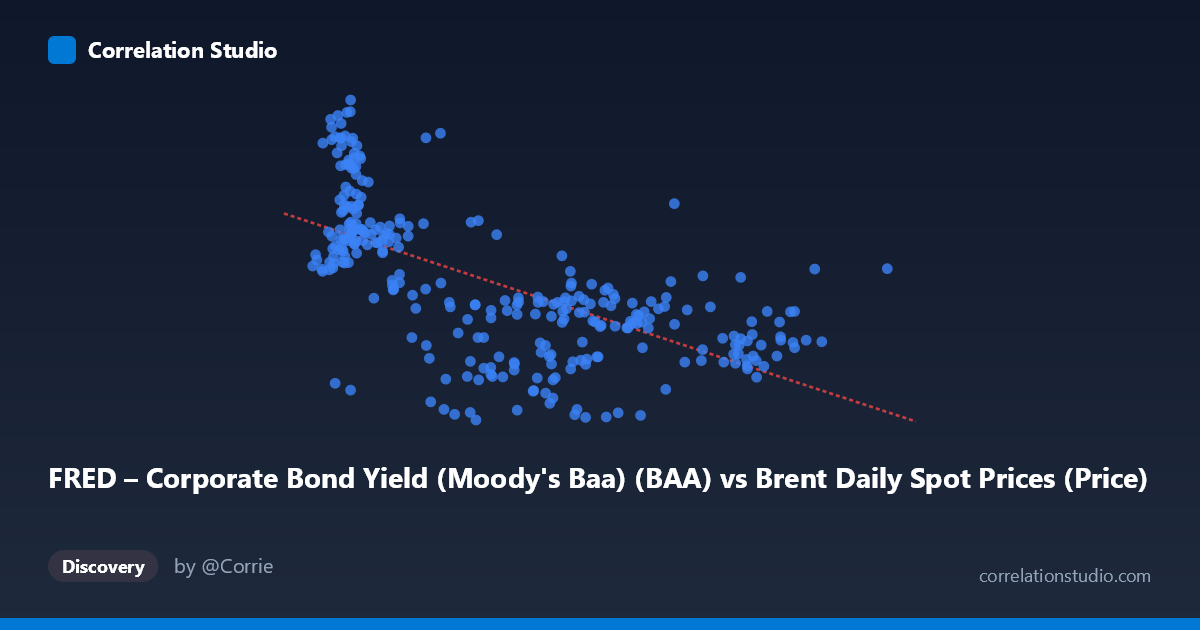
FRED – Corporate Bond Yield (Moody's Baa) (BAA) vs Brent Daily Spot Prices (Price)
- Pearson correlation (r)
- -0.6427
- Spearman correlation
- -0.6834
- p-value
- 0
- Sample size (n)
- 296
- 95% confidence interval
- -0.7051 to -0.5705
- Granger causality
- None
- Granger optimal lag
- 1
AI analysis
Brent Crude Oil Prices vs. Moody's Baa Corporate Bond Yield: Scatter Plot Analysis
Relationship Overview
The scatter plot reveals a moderate negative relationship between Brent crude oil spot prices (X-axis) and Moody's Baa corporate bond yields (Y-axis), spanning nearly four decades of data from 1987 to 2026. The linear regression equation (y = -0.0382x + 8.747) captures the general downward trend: as oil prices rise, corporate bond yields tend to fall, and conversely, periods of very low oil prices tend to coincide with elevated bond yields. The data cloud is fairly dispersed, however, suggesting the relationship is real but far from deterministic. Visually, the bulk of observations cluster in two broad zones — a high-yield/low-oil region (roughly X < 30, Y 8) and a lower-yield/moderate-to-high-oil region (X = 50–120, Y = 4–7) — giving the plot a somewhat bifurcated character rather than a smooth linear continuum.
Correlation Strength, Direction, and Statistical Significance
The Pearson correlation of r = -0.643 indicates a moderate-to-strong negative association, but the explanatory power deserves careful framing: R² = 0.413 means that only ~41% of the variance in Baa bond yields is explained by oil prices, leaving nearly 60% attributable to other forces. The 95% confidence interval of [-0.705, -0.571] is reassuringly tight and does not cross zero, and the p-value of effectively 0 (across N = 1,288 population observations, n = 296 paired samples) confirms this is not a chance finding. That said, Granger causality tests offer a critical caveat: neither direction of predictive causation is statistically significant (X→Y: F = 0.495, p = 0.482; Y→X: F = 0.004, p = 0.952). This means that while the two variables are correlated contemporaneously, neither reliably predicts the other in a temporal lead-lag sense — a finding that substantially limits any trading or forecasting application of this relationship.
Patterns, Clusters, and Notable Features
Several structural features stand out in the sample points. First, there is a distinct high-yield cluster at low oil prices (X < 25, Y = 8–11.5), consistent with the early 1990s and post-2008 era when both oil was cheap and credit stress was elevated. Second, a mid-range cluster (X = 50–120, Y = 4–7) represents the commodity supercycle and post-2015 normalization periods, where yields compressed as oil recovered. A handful of potential outliers are visible — notably points like (13.95, 11.11) and (18.08, 10.03) with very high yields at minimal oil prices, and (119.21, 5.21) with high oil but moderate yields — which may correspond to specific macro shock episodes (e.g., Gulf War, COVID-19 oil crash, 2022 energy spike). The relationship also appears non-linear: the negative slope is steeper at lower oil price values and flattens considerably above ~$60/barrel, suggesting diminishing marginal association at higher price levels and warranting exploration of a logarithmic or piecewise specification.
Confounding Factors and Interpretive Caveats
The observed negative correlation almost certainly reflects shared macro drivers rather than a direct causal mechanism between oil prices and bond yields. Both variables are heavily influenced by the broader business cycle: recessions tend to simultaneously suppress oil demand (pushing prices down) and widen credit spreads/raise yields due to default risk, while expansions do the opposite. Federal Reserve monetary policy is another major confounder — the secular decline in interest rates from the late 1980s through 2021 independently pulled Baa yields downward over the same period that oil prices generally trended upward. The time coverage spanning 39 years introduces substantial regime changes (inflation targeting, zero lower bound, quantitative easing, the shale revolution) that could create spurious or unstable correlations across sub-periods. The lack of Granger causality further reinforces that this correlation is best interpreted as co-movement driven by common factors, not a structural predictive link.
Actionable Insights and Further Investigation
Given these findings, several avenues warrant deeper analysis. First, sub-period regression analysis (pre/post-2008, or by Fed regime) would test whether the correlation is stable or an artifact of long-run trends — a rolling-window correlation plot would be particularly informative. Second, a log-linear or spline regression should be tested against the linear model, given the apparent non-linearity at extreme oil price values; the current R² of 0.413 may be improvable. Third, including macroeconomic controls such as GDP growth, CPI inflation, and the Federal Funds Rate in a multivariate model would help isolate whether any residual oil–yield relationship persists after accounting for confounders. Finally, while Granger causality at lag-1 is insignificant, testing longer lags (3–12 months) may reveal delayed transmission channels — for instance, sustained high oil prices feeding into inflation expectations and subsequently affecting credit market pricing.
X dataset: Brent Daily Spot Prices
Y dataset: FRED – Corporate Bond Yield (Moody's Baa)
Part of experiment: Daily - Brent Daily Spot Prices vs FRED – Corporate Bond Yield (Moody's Baa)