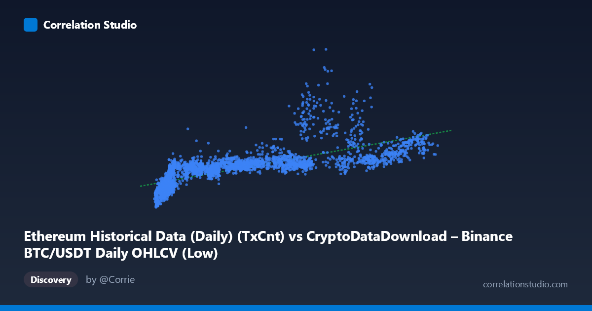
Ethereum Historical Data (Daily) (TxCnt) vs CryptoDataDownload – Binance BTC/USDT Daily OHLCV (Low)
- Pearson correlation (r)
- 0.7271
- Spearman correlation
- 0.879
- p-value
- 0
- Sample size (n)
- 3191
- 95% confidence interval
- 0.7103 to 0.743
- Granger causality
- None
- Granger optimal lag
- 10
- Time coverage
- 2017-08-17 to 2026-05-20
AI analysis
Analysis: Ethereum Transaction Count vs. Bitcoin Price (Low)
1. What the Visualization Reveals
Despite the mismatched labels (the axis metadata appears swapped—X is described as Ethereum TxCnt, Y as BTC/USDT Low), the underlying relationship is between a network activity metric and an asset price metric across a ~9-year span (2017–2026). The scatterplot shows a positive, moderately strong association: as the X-variable increases, Y tends to rise as well, but with substantial scatter rather than a tight linear band. The data suggests two variables that are broadly co-trending—likely both reflecting the general growth and cyclical boom/bust pattern of the crypto market—rather than one directly and mechanically determining the other.
2. Strength, Direction, and Uncertainty
The Pearson correlation (r = 0.727) indicates a moderately strong positive linear relationship, with r² = 0.529 meaning only about 53% of the variance in Y is explained by X — leaving nearly half unexplained by a linear model. The 95% CI [0.710, 0.743] is tight, and the p-value ≈ 0 confirms this correlation is highly unlikely due to chance, which is expected given the large sample (n = 3,191) and the fact that both series share a common trend over time (autocorrelated/non-stationary data inflates significance).
Critically, the Granger causality tests show no significant predictive direction in either direction (X→Y: p = 0.396; Y→X: p = 0.606). This means neither variable's past values help forecast the other's future values beyond what the series' own history provides. Practically: this is very likely a case of two trending time series that are correlated in level but not causally linked in a temporal/predictive sense — a classic contemporaneous co-movement without lead-lag structure.
3. Notable Patterns and Non-linear Features
The sample points show a distinctive fan/wedge shape: at low X values (~3,000–10,000), Y is tightly clustered in a lower band (~300K–1.1M), but as X grows past ~60,000, Y spreads out dramatically (1.2M to 3.6M+), with several high-leverage outliers (e.g., X≈65,712 paired with Y≈2.43M; X≈76,320 with Y≈2.9M). This heteroscedastic "trumpet" pattern — increasing variance at higher X — is a strong indicator of non-linearity. The note that Spearman ρ exceeds Pearson r reinforces this: the relationship is monotonic but not well-captured by a straight line, suggesting log-linear or power-law scaling (common in crypto metrics that grow multiplicatively).
4. Confounding Factors and Caveats
- Shared macro trend / time confound: Both variables likely trended upward over the 2017–2026 window due to overall crypto market growth, bull/bear cycles, and adoption — inflating the correlation without implying direct causation. - Non-stationarity: Neither series is likely stationary; computing Pearson r on trending series can produce "spurious regression" artifics. The Granger test (which typically differences/detrends) finding no causality supports this concern. - Label ambiguity: The stated axis descriptions conflict (X described as TxCnt, but sample values ~3,000–123,000 look like it could be daily transaction counts scaled oddly, while Y ranging into millions looks like price in USD — but the dataset names are cross-listed). This should be verified before drawing domain conclusions. - Outliers/regime shifts: Large deviations at high-X values may correspond to specific volatile periods (e.g., 2021 bull run, 2024 halving cycle) that disproportionately affect the linear fit.
5. Actionable Insights
- Refit with a log or power-law model (e.g., log(Y) ~ log(X)) given the Spearman/Pearson gap and fan-shaped variance — this will likely improve explained variance substantially. - Detrend or difference both series (e.g., use % changes or first differences) before assessing correlation/causality to rule out spurious trend-driven correlation. - Segment by market regime (bull vs. bear periods) to see if the relationship strength or slope changes — the wide scatter at high X suggests regime-dependent behavior. - Verify axis/data labeling to ensure the causal story (e.g., network usage driving price, or vice versa) is being tested on the correct variables. - Given the null Granger result, treat this as a descriptive correlation only — do not use one metric to forecast the other in a trading or predictive model without further validation (e.g., cointegration testing, VAR with additional lags/controls).
X dataset: CryptoDataDownload – Binance BTC/USDT Daily OHLCV
Y dataset: Ethereum Historical Data (Daily)
Part of experiment: Bitcoin - CryptoDataDownload – Binance BTC/USDT Daily OHLCV vs Ethereum Historical Data (Daily)