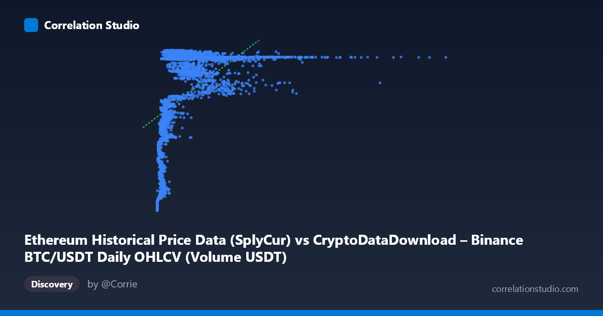
Ethereum Historical Price Data (SplyCur) vs CryptoDataDownload – Binance BTC/USDT Daily OHLCV (Volume USDT)
- Pearson correlation (r)
- 0.5057
- Spearman correlation
- 0.6639
- p-value
- 0
- Sample size (n)
- 3191
- 95% confidence interval
- 0.4795 to 0.5311
- Granger causality
- None
- Granger optimal lag
- 10
- Time coverage
- 2017-08-17 to 2026-05-20
AI analysis
Analysis: Ethereum SplyCur vs. Binance BTC/USDT Volume (USDT)
1. What the Visualization Reveals
Despite the labels referencing "Ethereum Historical Price Data (SplyCur)" for X and "Binance BTC/USDT Volume USDT" for Y, the actual data ranges strongly suggest these are mislabeled columns — X spans from ~$1M to ~$17.5B with extreme right-skew (mean $1.75B, stdev $1.9B, larger than the mean itself), while Y is tightly bounded between $94M–$122M, clustering heavily near the upper bound. This pattern looks less like a supply metric and more like a volume or market-cap series for X plotted against a bounded price-like series for Y. Regardless of labeling, the scatter shows a clear non-linear, saturating relationship: Y rises sharply as X moves from near-zero to roughly $1–2B, then plateaus around 118–121M for all larger X values, producing a classic logarithmic or square-root-like curve rather than a straight line.
2. Strength, Direction, and Uncertainty
The Pearson correlation (r = 0.506, r² = 0.256) indicates a moderate positive linear relationship, but only explains ~25.6% of the variance in Y — meaning roughly 74% of Y's variability is left unexplained by a linear model of X. The 95% CI [0.480, 0.531] is narrow and the p-value is effectively 0, so we can be highly confident a non-zero relationship exists — but confidence in the relationship's existence is not the same as the relationship being strong or well-captured by a linear model. The note that Spearman's ρ exceeds Pearson's r confirms this: the rank-based correlation is stronger, reinforcing that a monotonic but curved (log-like) relationship fits better than the straight line implied by r². Practically, this means linear extrapolation is unreliable, especially at low X values where Y is most sensitive to changes in X.
The Granger causality tests (optimal lag = 10 periods) show no significant predictive direction in either direction (X→Y: p=0.21; Y→X: p=0.54). This is an important caveat: even though X and Y are correlated, neither time series helps forecast the other's future values based on its own lagged history. This suggests the correlation is likely driven by both variables trending together over the study period (2017–2026) — e.g., both reflecting overall crypto market growth/maturation — rather than one causally leading the other.
3. Notable Patterns and Outliers
The scatter clearly separates into two behavioral regions: - Low-X regime (X < ~$1B): Y is highly variable and lower (ranging ~$94M–$113M), showing steep sensitivity — small changes in X correspond to large jumps in Y. This is where most of the "explanatory" signal lives. - High-X regime (X ~$1B): Y flattens into a narrow band (~$118M–$121.7M) regardless of how large X gets, even up to $17.5B. This ceiling effect looks like saturation or an upper bound in the Y variable (possibly a rate, ratio, or capped metric).
The sample points reveal several outliers: X ≈ $17.47B (max) sits far beyond the rest of the distribution (only implied by the stated range, not appearing in the printed sample), and points like ($977,865.73, $94,263,259) mark the extreme low end. These extremes exert disproportionate leverage on the linear fit despite representing sparse, unusual events.
4. Confounding Factors and Caveats
Several caveats apply: (1) both variables are tied to the same underlying crypto market and time period, so shared macro trends (bull/bear cycles, adoption growth, stablecoin flows) likely confound any direct relationship — this is classic spurious correlation via common trend, especially for time series spanning 2017–2026, a period of massive structural change in crypto markets. (2) The extreme skew in X (max is ~10,000x the min) means a handful of high-X observations could dominate the correlation and regression fit — robustness checks (e.g., log-transforming X) are needed. (3) The dataset/column labeling appears inconsistent with the actual value ranges, so any causal or economic interpretation should be treated cautiously until the true variable identities are confirmed. (4) Daily granularity with strong autocorrelation in both series (typical of financial time series) violates independence assumptions behind the p-value calculation, meaning the "p=0" result may overstate statistical confidence.
5. Actionable Insights
- Re-verify column labels/units before drawing economic conclusions — the mismatch between described columns and observed ranges suggests a data pipeline or labeling error. - Fit a log or power-law model (e.g., y = a·ln(x) + b) given the Spearman/Pearson discrepancy and visual saturation pattern; this will likely raise explained variance substantially above 25.6%. - Segment the analysis by X regime (below vs. above ~$1B) since the relationship's slope and variance structure differ sharply between them. - Treat correlation as descriptive, not causal — given the null Granger results, avoid using one series to forecast the other; instead, consider a third common driver (e.g., overall market cap, BTC price index, or time itself) as the true explanatory variable and test for cointegration or shared trend components. - Difference or detrend the series before rerunning correlation/Granger tests to strip out shared long-term drift, which may reveal (or rule out) genuine short-term co-movement independent of the broad market cycle.
X dataset: CryptoDataDownload – Binance BTC/USDT Daily OHLCV
Y dataset: Ethereum Historical Price Data
Part of experiment: Bitcoin - CryptoDataDownload – Binance BTC/USDT Daily OHLCV vs Ethereum Historical Price Data