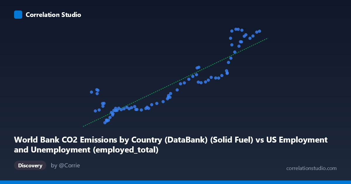
World Bank CO2 Emissions by Country (DataBank) (Solid Fuel) vs US Employment and Unemployment (employed_total)
- Pearson correlation (r)
- 0.9019
- Spearman correlation
- 0.8709
- p-value
- 0
- Sample size (n)
- 80
- 95% confidence interval
- 0.8508 to 0.9361
- Granger causality
- None
- Granger optimal lag
- 10
- Time coverage
- 1941-01-01 to 2020-01-01
AI analysis
Scatterplot Analysis: US Total Employment vs. CO2 Solid Fuel Emissions
1. Overall Relationship
The scatterplot reveals a strong, positive linear relationship between solid fuel CO2 emissions and total US employment across the 1941–2020 period. As solid fuel emissions increase (X-axis, ranging from ~50,350 to ~157,538 units), total employment rises correspondingly (Y-axis, ~9,555 to ~31,154 units). The fitted regression line (y = 0.173x + 877.3) captures this trend well, suggesting that for every unit increase in solid fuel emissions, employment rises by approximately 0.173 units on average. Both variables almost certainly reflect the same underlying driver — long-run economic and demographic growth — which produces this apparently tight co-movement over eight decades of annual data.
2. Correlation Strength and Statistical Interpretation
The Pearson correlation of r = 0.902 is very strong, and the coefficient of determination R² = 0.813 indicates that roughly 81.3% of the variance in total employment is statistically accounted for by solid fuel emissions within this sample. The 95% confidence interval for r of [0.851, 0.936] is narrow and lies entirely in high-positive territory, reflecting reliable estimation across the n = 80 paired observations. The p-value of essentially zero confirms this association is not a sampling artifact. However, the Granger causality results are notably non-significant in both directions (X→Y: F = 1.07, p = 0.399; Y→X: F = 1.10, p = 0.378) at the optimal lag of 10 periods. This means neither variable meaningfully predicts future changes in the other beyond what each already contains, strongly implying that the correlation reflects shared common trends rather than any directional causal mechanism.
3. Patterns, Clusters, and Outliers
The data broadly separate into two visible clusters: a lower-left cluster (X < ~90,000; Y < ~15,000) corresponding to earlier decades with lower emissions and smaller labor forces, and an upper-right cluster (X ~120,000; Y ~18,000) representing later decades with expanded emissions and employment. The transition zone between roughly X = 90,000–120,000 appears somewhat less densely populated, possibly reflecting mid-century structural transitions. Several points in the lower-left deviate noticeably from the regression line — for example, points near (50,350; 16,616), (53,750; 17,184), and (53,960; 16,275) show surprisingly high employment relative to their low emissions values, suggesting these may correspond to wartime or early post-war anomalies where employment surged while coal-heavy emissions had not yet caught up. Conversely, a few upper-range points (e.g., (142,469; 31,154) and (145,362; 28,261)) show some scatter around the line, hinting at mild heteroscedasticity at higher values.
4. Confounding Factors and Caveats
The most critical caveat is that both variables are non-stationary time series with shared secular upward trends — population growth, GDP expansion, and industrialization drive both employment totals and fossil fuel consumption simultaneously, creating a spurious correlation scenario. The Granger causality failure makes this explicit: there is no evidence of temporal predictive power between them. Additionally, the dataset labeling appears inverted (the X-axis is described as coming from a US Employment dataset while the Y-axis comes from a CO2 dataset), which warrants careful verification before drawing any domain conclusions. Energy mix shifts — such as the post-2000 decline in coal relative to natural gas — may also distort the solid-fuel-specific relationship in later years, contributing to upper-range scatter. Finally, using annual aggregates masks within-year dynamics and cyclical fluctuations (e.g., recessions) that could alter the apparent relationship substantially.
5. Actionable Insights and Further Investigation
Given that the strong correlation almost certainly reflects common trend confounding rather than genuine causality, analysts should detrend or difference both series before drawing any policy-relevant conclusions — examining whether changes in solid fuel emissions predict changes in employment would be far more informative. It would also be valuable to extend the Granger causality test across multiple lag structures beyond 10 periods and to apply cointegration tests (e.g., Engle-Granger or Johansen) to determine whether a stable long-run equilibrium relationship actually exists. Segmenting the analysis by era (pre-/post-1970 energy crisis; pre-/post-2008 shale revolution) could reveal whether the relationship has been structurally stable or has shifted. Finally, controlling for GDP or population as explicit confounders would help isolate whether any residual employment–emissions relationship persists after removing the dominant shared growth trend.
X dataset: US Employment and Unemployment
Y dataset: World Bank CO2 Emissions by Country (DataBank)
Part of experiment: Yearly - US Employment and Unemployment vs World Bank CO2 Emissions by Country (DataBank)