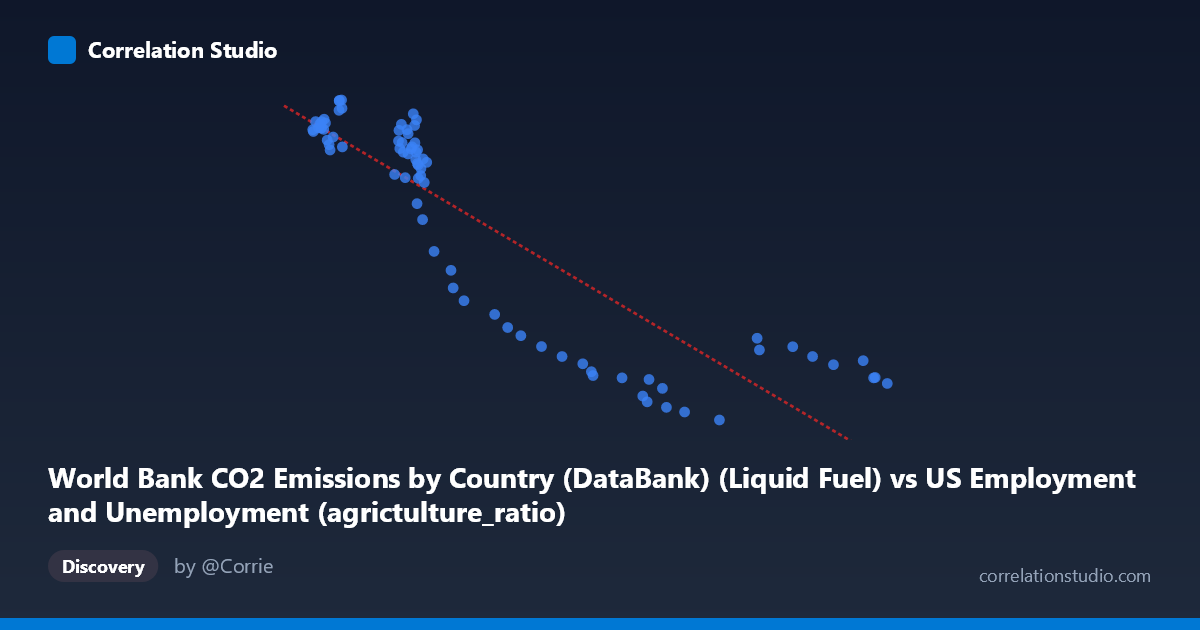
World Bank CO2 Emissions by Country (DataBank) (Liquid Fuel) vs US Employment and Unemployment (agrictulture_ratio)
- Pearson correlation (r)
- -0.8826
- Spearman correlation
- -0.89
- p-value
- 0
- Sample size (n)
- 80
- 95% confidence interval
- -0.9233 to -0.8224
- Granger causality
- None
- Granger optimal lag
- 10
AI analysis
Scatterplot Analysis: Liquid Fuel CO2 Emissions vs. US Agricultural Employment Ratio
1. Overall Relationship
The scatterplot reveals a strong negative relationship between World Bank liquid fuel CO2 emissions and the US agricultural employment ratio over the period 1941–2020. As liquid fuel CO2 emissions increase, the proportion of the US workforce engaged in agriculture declines markedly. The linear regression equation (y = −1.648x + 16,267.3) captures this inverse trend well, suggesting that for every unit increase in liquid fuel emissions, the agricultural employment ratio drops by approximately 1.65 units. This pattern is consistent with a broader narrative of post-war industrialization and economic modernization: as fossil fuel consumption expanded to power mechanized agriculture and broader economic activity, fewer workers were needed on farms.
2. Correlation Strength, Direction, and Temporal Causality
The Pearson correlation of r = −0.883 indicates a strong negative association, and the R² of 0.779 means that roughly 77.9% of the variance in the agricultural employment ratio is statistically explained by liquid fuel CO2 emissions — a substantial figure for a real-world social and economic relationship. The 95% confidence interval of [−0.923, −0.822] is tight and entirely negative, reinforcing that this inverse relationship is unlikely to be a statistical artifact, and the p-value of essentially 0 confirms it is highly significant at any conventional threshold. However, the Granger causality results complicate any directional interpretation: neither X→Y (F = 1.19, p = 0.321) nor Y→X (F = 1.46, p = 0.182) achieves significance, even at an optimal lag of 10 periods. This means that, despite the strong contemporaneous correlation, neither variable reliably predicts the future movement of the other in a time-series sense. The variables move together historically but do not temporally lead or lag each other in a statistically meaningful way.
3. Notable Patterns, Clusters, and Outliers
The scatterplot displays a visibly curved or heteroscedastic structure rather than a perfectly linear spread. At low X values (roughly 2,095–3,500), Y values cluster densely between approximately 10,000 and 13,600, suggesting a plateau or saturation region where high agricultural ratios were common during the early decades of the dataset. As X increases beyond ~4,000–5,000, Y drops sharply and then appears to level off again at the lower end (3,000–5,500 range), hinting at a potential non-linear, possibly exponential decay relationship. Several points at high X values (e.g., 9,250; 9,100; 9,080) show Y values clustering tightly around 3,800–4,600, forming a lower-right cluster. The point at (7,160; 2,497) appears as a potential low outlier, with Y well below the trend for its X range, which may reflect an anomalous year worth investigating. The dense cluster in the low-X, high-Y region (pre-1970s era) versus the sparse spread in the high-X region (post-1980s) also indicates uneven temporal sampling or acceleration in emissions in later decades.
4. Confounding Factors and Interpretive Caveats
The most critical caveat is that both variables are strongly driven by time itself — this is almost certainly a case of spurious correlation mediated by a shared temporal trend. US agricultural employment declined monotonically due to mechanization, rural-to-urban migration, and structural economic change, while global liquid fuel CO2 emissions rose due to industrialization, transportation growth, and population increase. These two trends share a common driver (the passage of time and economic development) but are not necessarily causally linked to each other. The failure of Granger causality tests supports this interpretation. Additionally, the X-axis variable is labeled as coming from a US Employment dataset but describes World Bank CO2 emissions — this cross-dataset join introduces potential measurement inconsistencies, aggregation mismatches, and definitional ambiguities. The "liquid fuel" subcategory of CO2 also represents only one emissions source, and its relationship to US agricultural ratios specifically (rather than global or US-only emissions) is conceptually indirect.
5. Actionable Insights and Further Investigation
Given the strong but likely time-mediated correlation, the most important next step is to partial out the effect of time by regressing both variables on year and examining the residuals, or by using first-differenced series to test whether changes in emissions predict changes in agricultural employment independently of trend. Researchers should also explore non-linear model fits (e.g., logarithmic or power-law regression), which may better capture the apparent curvature in the scatterplot and improve upon the already high R² of 0.779. It would be valuable to disaggregate the data by decade to see whether the relationship holds consistently across historical periods or whether it was driven primarily by the 1940s–1970s structural transition. Investigating alternative confounders — GDP per capita, agricultural mechanization indices, rural population share, or total energy consumption — would help isolate whether any direct mechanism exists. Finally, the apparent outlier near (7,160; 2,497) should be examined for data quality or whether it represents a structurally unusual year (e.g., wartime disruption, economic recession) that merits separate treatment.
X dataset: US Employment and Unemployment
Y dataset: World Bank CO2 Emissions by Country (DataBank)
Part of experiment: Yearly - US Employment and Unemployment vs World Bank CO2 Emissions by Country (DataBank)