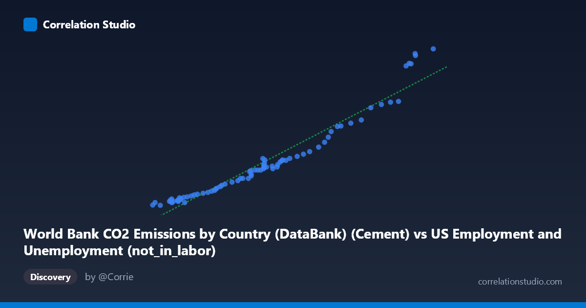
World Bank CO2 Emissions by Country (DataBank) (Cement) vs US Employment and Unemployment (not_in_labor)
- Pearson correlation (r)
- 0.9687
- Spearman correlation
- 0.9898
- p-value
- 0
- Sample size (n)
- 80
- 95% confidence interval
- 0.9516 to 0.9799
- Granger causality
- None
- Granger optimal lag
- 10
- Time coverage
- 1941-01-01 to 2020-01-01
AI analysis
Scatterplot Analysis: Cement CO2 Emissions vs. US Labor Force Non-Participation
1. Overall Relationship Pattern
The scatterplot reveals a strong, positive, approximately linear relationship between World Bank cement-related CO2 emissions and the US "not in labor force" population count. As cement CO2 emissions increase from roughly 38,590 to 99,587 (units), the not-in-labor-force figure rises correspondingly from approximately 79 to 2,609 (units). The data points follow the regression line y = 0.0387x − 1648.91 quite closely across most of the range, suggesting a remarkably consistent co-movement spanning the 1941–2020 time period covered by this dataset. The relationship appears predominantly linear, with perhaps slight curvature at the upper end where high-emission observations cluster near values exceeding 90,000.
2. Correlation Strength and Statistical Framing
The Pearson correlation of r = 0.9687 is exceptionally high, and the R² of 0.9385 means that approximately 93.8% of the variance in the not-in-labor-force measure is statistically explained by the linear model using cement CO2 emissions as the predictor. The 95% confidence interval for r of [0.9516, 0.9799] is narrow and situated entirely in the strong-positive region, indicating high precision in the correlation estimate across the n = 80 paired observations. The p-value of effectively zero confirms this association is statistically significant far beyond conventional thresholds. However, the Granger causality results are notably unimpressive: neither direction (X→Y: F = 0.347, p = 0.963; Y→X: F = 0.628, p = 0.783) approaches significance even at the optimal lag of 10 periods. This means that despite the near-perfect contemporaneous correlation, neither variable temporally predicts the other — a critical finding that strongly argues against any causal interpretation.
3. Notable Patterns, Clusters, and Outliers
The data naturally segments into at least two visible clusters: a dense lower-left cluster (X ≈ 38,000–65,000; Y ≈ 80–850) representing earlier decades of the time series, and a sparser upper-right cluster (X ≈ 80,000–99,600; Y ≈ 1,400–2,610) representing more recent high-emission, high-non-participation periods. The uppermost observations — particularly the point near (99,587; 2,609) and several clustered near (93,000–96,000; 2,330–2,530) — sit at the extreme of the range and could be influential leverage points in the regression. A few points in the middle range (e.g., around X ≈ 62,000–63,000) show modest scatter around the regression line, suggesting some heteroscedasticity where variance in Y increases at higher X values, which is consistent with what one might expect when both series grow over time.
4. Confounding Factors and Critical Caveats
The most important caveat here is the classic spurious correlation driven by shared secular time trends. Both variables — global cement CO2 emissions and the US not-in-labor-force population — have grown substantially over the eight decades from 1941 to 2020, largely driven by independent processes: global industrialization and population growth in one case, and US demographic aging, baby boomer retirement, and workforce participation shifts in the other. When two time series both trend upward over the same period, they will almost always yield high correlations regardless of any mechanistic connection. The datasets themselves reinforce this concern: cement CO2 comes from a global World Bank dataset, while the labor force variable is US-specific — there is no plausible direct mechanism linking global cement production to American labor non-participation. The absence of Granger causality in either direction provides the statistical confirmation of this suspicion.
5. Actionable Insights and Further Investigation
The near-zero Granger causality p-values should be treated as the most actionable finding: do not use this correlation to justify any policy or causal claim. For rigorous analysis, both series should be detrended (e.g., via first-differencing or HP filtering) before computing correlations, which would almost certainly collapse the r value dramatically. Researchers should investigate whether a spurious regression is occurring by performing cointegration tests (e.g., Engle-Granger or Johansen), which would determine whether any long-run equilibrium relationship exists beyond shared trending. If the goal is understanding drivers of US labor non-participation, far more theoretically grounded predictors — such as aging demographics, disability rates, educational enrollment, or wage levels — should be prioritized. Similarly, cement CO2 drivers are better explored through construction activity indices, GDP, or urbanization rates. This analysis serves as a compelling classroom example of why correlation, even at r = 0.97, explains nothing without causal mechanism and temporal precedence.
X dataset: US Employment and Unemployment
Y dataset: World Bank CO2 Emissions by Country (DataBank)
Part of experiment: Yearly - US Employment and Unemployment vs World Bank CO2 Emissions by Country (DataBank)