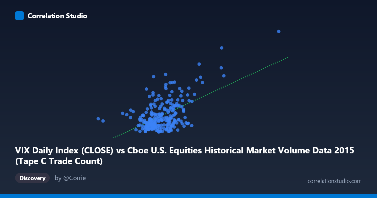
VIX Daily Index (CLOSE) vs Cboe U.S. Equities Historical Market Volume Data 2015 (Tape C Trade Count)

Pearson correlation (r): 0.5495
Spearman correlation: 0.3537
p-value: 0
Sample size (n): 252
95% confidence interval: 0.457 to 0.6303
Granger causality: None
Granger optimal lag: 1

AI analysis

Analysis: VIX Daily Index vs. Tape C Trade Count (2015)

Relationship Overview The scatterplot reveals a moderate positive relationship between the Cboe VIX Daily Index (close) and Tape C Trade Count across U.S. equity exchanges in 2015. As market volume (X) increases, VIX levels (Y) tend to rise correspondingly, which aligns intuitively with market microstructure theory: higher trading activity is often associated with elevated uncertainty and volatility. The linear regression equation (y = 1.81×10⁻⁵x + 2.975) confirms this upward slope, though the intercept suggests a baseline VIX level even at minimal trading volumes. The relationship is broadly linear across the central range of observations but shows increasing dispersion at higher volume levels, hinting at heteroscedasticity.

Correlation Strength and Statistical Significance The Pearson correlation of r = 0.5495 indicates a moderate positive association, but the r² of 0.3020 is the more practically informative figure — it means that only 30.2% of the variance in VIX levels is explained by Tape C trade count, leaving nearly 70% of VIX variability attributable to other factors. The 95% confidence interval for r [0.4570, 0.6303] is reasonably tight given the sample size of n = 252, and the p-value of effectively zero confirms this is not a chance finding across the N = 3,302 population. However, statistical significance should not be conflated with practical importance: the relationship is real but far from deterministic. Critically, Granger causality tests show no significant directional predictive relationship in either direction (X→Y: F = 0.0496, p = 0.824; Y→X: F = 0.1332, p = 0.715), meaning that neither variable reliably predicts the other's future values at a one-period lag. This strongly cautions against any causal or predictive interpretation of the correlation.

Notable Patterns, Clusters, and Outliers The sample data reveals several structural features worth noting. The bulk of observations cluster between approximately 600,000–900,000 in trade count and 12–22 in VIX, forming a dense central core. However, there are clear high-leverage outliers — most notably the point near (1,194,528, 36.02) and another near (1,210,006, 28.03), representing days of extreme trading volume coinciding with elevated VIX readings. These likely correspond to the August 2015 market selloff, a well-documented volatility spike. The point at (291,078, 15.74) is an extreme outlier on the low-volume end, suggesting a possible holiday-shortened trading session or data anomaly. There also appears to be a diffuse upper scatter band where moderate volumes (~700,000–800,000) correspond to surprisingly elevated VIX readings (e.g., 24–28), suggesting the relationship is not uniformly linear.

Confounding Factors and Caveats Several important caveats apply. First, reverse causality is plausible and perhaps more theoretically grounded — VIX spikes may drive trading volume rather than volume driving VIX — yet Granger tests refute even this directional framing at the one-period lag. Second, omitted variable bias is substantial: macroeconomic events, Federal Reserve announcements, earnings seasons, and global risk-off episodes all independently influence both variables simultaneously, potentially inflating the observed correlation. Third, the dataset spans only 2015 — a year with a specific volatility regime (relatively calm early year, sharp August shock) — which limits generalizability to other market environments. Fourth, using Tape C trade count specifically (NYSE Arca-listed securities) may not be representative of aggregate market behavior, introducing selection bias.

Actionable Insights and Further Investigation Given the moderate correlation and absence of Granger causality, practitioners should avoid using either variable as a standalone leading indicator for the other. More productive next steps would include: (1) extending the analysis across multiple years (2010–2023) to test whether the r ≈ 0.55 relationship holds across different volatility regimes; (2) decomposing the August 2015 outlier period separately to assess whether the correlation is primarily regime-driven rather than structural; (3) introducing multivariate controls such as S&P 500 returns, bid-ask spreads, or options open interest to better isolate the trade count–VIX channel; and (4) testing non-linear models (e.g., log-log or polynomial regression) given the apparent heteroscedasticity at high volumes. The strong clustering in the data also suggests that regime-switching models or quantile regression may reveal richer conditional relationships than a single OLS fit captures.

X dataset: Cboe U.S. Equities Historical Market Volume Data 2015

Y dataset: VIX Daily Index

Part of experiment: Daily - Cboe U.S. Equities Historical Market Volume Data 2015 vs VIX Daily Index