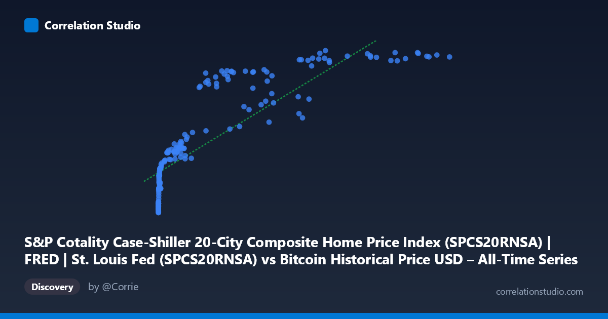
S&P Cotality Case-Shiller 20-City Composite Home Price Index (SPCS20RNSA) | FRED | St. Louis Fed (SPCS20RNSA) vs Bitcoin Historical Price USD – All-Time Series (Habrador) (Price)
- Pearson correlation (r)
- 0.8491
- Spearman correlation
- 0.9706
- p-value
- 0
- Sample size (n)
- 189
- 95% confidence interval
- 0.8038 to 0.8846
- Granger causality
- None
- Granger optimal lag
- 9
AI analysis
Analysis: Bitcoin Price vs. Case-Shiller Home Price Index
1. What the Visualization Reveals
The scatterplot depicts a strong positive association between Bitcoin's historical USD price (X-axis) and the S&P Case-Shiller 20-City Composite Home Price Index (Y-axis). Despite these being fundamentally unrelated economic series — one a volatile cryptocurrency valued in nominal dollars, the other a smoothed, inflation-linked housing index — the data trace a clear upward-sloping pattern. The relationship appears curved rather than strictly linear: at low Bitcoin prices (sub-$1,000), the Case-Shiller index clusters tightly between ~135-215, while as Bitcoin climbs into the tens of thousands, the index rises more gradually toward its 330-345 ceiling. This compressive, decelerating shape at high X-values is consistent with a logarithmic or power-law fit rather than a straight line.
2. Strength, Direction, and Statistical Caveats
The Pearson correlation (r = 0.849, r² = 0.721) indicates a strong positive linear relationship, with 72% of the variance in the housing index "explained" by Bitcoin's price in a purely statistical sense. The tight 95% confidence interval [0.804, 0.885] and p-value of 0 (effectively <0.001) suggest this correlation is highly unlikely to be due to random sampling noise. However, statistical significance here should not be conflated with causal or economically meaningful linkage. Critically, the Granger causality tests show no significant predictive direction in either direction (X→Y: p=0.608; Y→X: p=0.741) — neither series helps forecast the other's future movements once past values of each are accounted for. This is a strong signal that the correlation is not driven by one variable temporally leading the other, but likely reflects two series that are both trending upward over the same calendar period (2010-2026) for unrelated reasons.
3. Notable Patterns and Outliers
Several features stand out: (a) a dense cluster of low-X points (Bitcoin under $100) mapped to Y-values around 134-165, representing Bitcoin's early years (2010-2013) overlaid on a slowly recovering post-financial-crisis housing market; (b) a mid-range zone (X ≈ 1,000-10,000) where Y climbs from ~190 to ~215, coinciding with Bitcoin's 2017 boom and steady housing recovery; and (c) a high-X cluster (X 50,000) where Y plateaus near 330-345, corresponding to 2021-2024 when Bitcoin experienced huge volatility (crashes and rallies) while housing prices rose more steadily and then flattened. The flattening of Y at high X, despite continued X growth, produces the curvature that makes a log-transform of X likely to fit better (as hinted by Spearman ρ exceeding Pearson r).
4. Confounding Factors and Caveats
The most important caveat is shared temporal trend, not causation. Both series generally trended upward over 2010-2026 due to independent macro forces: Bitcoin's rise reflects adoption, speculation, and crypto-market cycles; the Case-Shiller index reflects low interest rates (until 2022), constrained housing supply, and general inflation. Since both are essentially time-indexed and non-stationary, any two upward-trending series over the same window will show spurious correlation — a classic time-series pitfall. Autocorrelation within each series (each observation resembles its neighbors) inflates the apparent r and understates true degrees of freedom, which is why the Granger test (which controls for each series' own lagged history) reveals no genuine predictive relationship. Macroeconomic conditions (Fed policy, inflation, liquidity) are the likely common confounders driving both variables simultaneously.
5. Suggestions for Further Investigation
Given the lack of Granger causality, this correlation should not be used for forecasting one asset from the other. To properly assess any real relationship, analysts should: (1) detrend or difference both series (e.g., use % changes or YoY growth rates rather than levels) and re-test correlation/Granger causality on the stationary series; (2) explicitly control for shared macro covariates like the Fed Funds rate, CPI, or M2 money supply, which plausibly drive both housing prices and speculative crypto demand; (3) fit and compare a log-linear or power model given the visual curvature and the Spearman/Pearson discrepancy; and (4) consider that with only 189 paired monthly observations exhibiting strong autocorrelation, effective sample size is much smaller than 189, warranting caution before drawing economic conclusions from the raw r² figure.
X dataset: Bitcoin Historical Price USD – All-Time Series (Habrador)
Y dataset: S&P Cotality Case-Shiller 20-City Composite Home Price Index (SPCS20RNSA) | FRED | St. Louis Fed
Part of experiment: Bitcoin - Bitcoin Historical Price USD – All-Time Series (Habrador) vs S&P Cotality Case-Shiller 20-City Composite Home Price Index (SPCS20RNSA) | FRED | St. Louis Fed