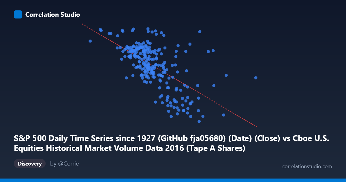
S&P 500 Daily Time Series since 1927 (GitHub fja05680) (Date) (Close) vs Cboe U.S. Equities Historical Market Volume Data 2016 (Tape A Shares)

Pearson correlation (r): -0.6197
Spearman correlation: -0.614
p-value: 0
Sample size (n): 252
95% confidence interval: -0.6904 to -0.5372
Granger causality: None
Granger optimal lag: 4

AI analysis

Analysis: S&P 500 Close Price vs. Cboe Tape A Share Volume (2016)

Relationship Overview The scatterplot reveals a negative relationship between the S&P 500 closing price (X-axis) and Cboe Tape A share volume (Y-axis) across 252 trading days in 2016. As the S&P 500 index level rises, Tape A share volume tends to decline, and conversely, lower index levels are associated with higher trading volumes. This inverse pattern is consistent with a well-documented market dynamic: elevated volatility and fear — typically coinciding with lower price levels — tend to drive higher trading activity, while calm, rising markets often see reduced participation and volume compression.

Correlation Strength and Statistical Significance The Pearson correlation of r = -0.6197 indicates a moderate-to-strong negative linear association. The R² of 0.384 means that approximately 38.4% of the variance in Tape A share volume is explained by the S&P 500 price level — a meaningful but far from complete relationship, leaving over 61% of volume variability unexplained by price alone. The 95% confidence interval of [-0.6904, -0.5372] is entirely negative and reasonably tight, confirming the direction with strong statistical certainty, and the p-value of ~0 leaves no doubt that this correlation is not a chance artifact given the population of N = 3,622. However, the Granger causality results tell a more cautionary tale: neither direction (X→Y nor Y→X) shows statistical significance at the optimal 4-period lag (F = 0.60, p = 0.66 for X→Y; F = 1.14, p = 0.34 for Y→X). This means that while the two variables are correlated contemporaneously, neither reliably predicts the other in a temporal, lead-lag sense — an important distinction between association and predictive causality.

Patterns, Clusters, and Outliers The scatterplot shows a recognizable funnel or wedge-shaped distribution when moving from lower to higher X values. Several features stand out: - A cluster of high-volume observations (Y 2150) concentrated in the X range of roughly 175M–265M, suggesting that lower index levels (likely early 2016 market stress) coincided with elevated Tape A activity - A cluster of lower-volume, higher-price observations in the X range of 290M–370M, consistent with the calmer, trending-upward second half of 2016 - Notable outliers include the point near (190M, 2265) — exceptionally high volume paired with a low price level — and (278M, 2262) — high volume despite a mid-range price, which deviates noticeably from the trend line and warrants further scrutiny - A sparse but visible tail of very high X values (above 400M) with moderate Y values suggests some high-close-price days with ordinary volume

Confounding Factors and Caveats Several important caveats apply to interpreting this correlation. First, 2016 was an unusual year with discrete macro shocks — the Brexit vote (June), U.S. election (November), and a sharp early-year selloff — each capable of simultaneously depressing prices and spiking volume independently. These events may inflate the observed correlation without reflecting a structural mechanism. Second, Tape A volume is only one component of total U.S. equity market volume; Tapes B and C, dark pools, and off-exchange activity may behave differently. Third, the linear regression model (y = -1.069e-6x + 2385.89) may oversimplify what appears to be a potentially non-linear or regime-dependent relationship — the scatter suggests heteroscedasticity, with variance in Y being larger at lower X values. Finally, reverse causality and confounding through volatility (VIX) is highly plausible: volatility likely drives both lower prices and higher volumes simultaneously, acting as a hidden common cause rather than price directly influencing volume.

Actionable Insights and Further Investigation Practitioners and researchers should consider several follow-up directions. Incorporating the VIX or realized volatility as a mediating or control variable would help decompose whether the price-volume relationship is direct or entirely mediated through volatility. Given the failed Granger causality tests, intraday data analysis might reveal shorter-term lead-lag dynamics that daily data obscures. It would also be valuable to test this relationship across multiple years to determine whether the 2016 pattern is structurally persistent or event-driven. For trading strategy development, the lack of Granger causality is a clear warning that this correlation cannot be naively exploited for predictive signals without additional conditioning variables. Finally, segmenting the data by market regime (e.g., pre/post-election, high/low VIX environments) could reveal whether the correlation strengthens or breaks down in specific contexts, offering more actionable and robust insights.

X dataset: Cboe U.S. Equities Historical Market Volume Data 2016

Y dataset: S&P 500 Daily Time Series since 1927 (GitHub fja05680) (Date)

Part of experiment: Daily - Cboe U.S. Equities Historical Market Volume Data 2016 vs S&P 500 Daily Time Series since 1927 (GitHub fja05680) (Date)