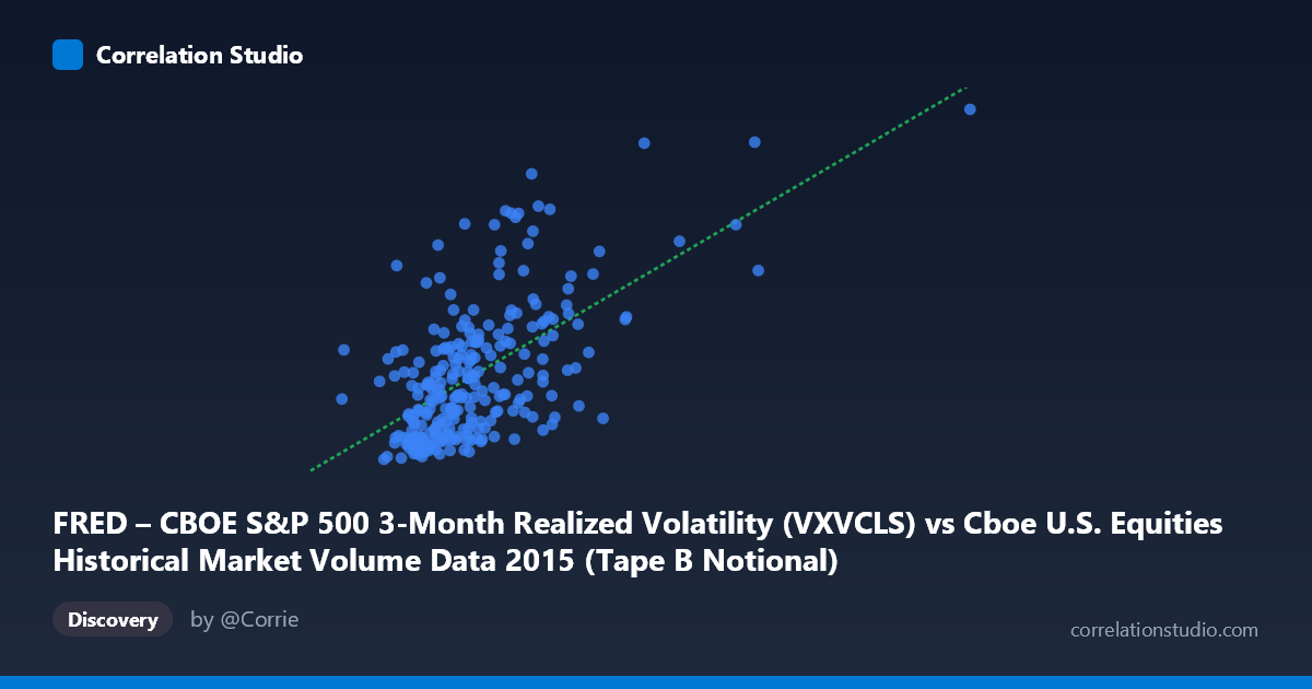
FRED – CBOE S&P 500 3-Month Realized Volatility (VXVCLS) vs Cboe U.S. Equities Historical Market Volume Data 2015 (Tape B Notional)
- Pearson correlation (r)
- 0.6031
- Spearman correlation
- 0.5451
- p-value
- 0
- Sample size (n)
- 252
- 95% confidence interval
- 0.5181 to 0.6762
- Granger causality
- None
- Granger optimal lag
- 1
AI analysis
Analysis: CBOE S&P 500 3-Month Realized Volatility vs. Tape B Notional Volume (2015)
Relationship Overview
The scatterplot reveals a moderate positive relationship between Cboe S&P 500 3-Month Realized Volatility (VXVCLS) and Tape B Notional trading volume across 2015 trading days. As realized volatility increases, Tape B notional value tends to rise as well, which aligns intuitively with market microstructure theory: elevated volatility environments typically generate heightened trading activity as market participants reposition, hedge, and respond to price uncertainty. The linear regression equation (y = 1.11×10⁻⁹x + 12.45) quantifies this upward slope, though the intercept near 12.45 suggests a meaningful baseline volatility level even at minimal volume.
Correlation Strength and Statistical Significance
The Pearson correlation of r = 0.6031 indicates a moderate-to-strong positive association, but the explanatory power is more soberly framed by r² = 0.3637 — meaning only 36.4% of the variance in volatility is explained by Tape B notional volume. The remaining ~64% is attributable to other factors entirely. The 95% confidence interval of [0.5181, 0.6762] is relatively tight given n = 252, and the p-value of effectively zero confirms this correlation is highly unlikely to be a chance artifact. However, the Granger causality tests tell a critical story: neither direction (X→Y nor Y→X) achieves significance (F = 0.0076, p = 0.93 and F = 0.0222, p = 0.88 respectively). This means that despite the contemporaneous correlation, neither variable reliably predicts the other in the next period — the relationship is associative but not temporally predictive at a 1-day lag.
Patterns, Clusters, and Outliers
Several notable structural features emerge from the sample points. The bulk of observations cluster in the lower-left region (volume roughly 3–6 billion, volatility 14–21), suggesting that most 2015 trading days were characterized by moderate activity. However, there is a meaningful dispersion tail extending toward higher volatility readings (25–31), often associated with larger volume figures — points such as (12,491,974,395; 29.58) and (6,892,776,331; 28.07) stand out as potential high-stress market days. The wide X-axis range (2.1B to 17.9B) relative to the dense core cluster suggests occasional extreme volume days, possibly tied to specific macro events like the August 2015 volatility spike. The relationship also appears to fan outward at higher volume levels, hinting at heteroscedasticity where volatility becomes harder to predict at extreme volume.
Confounding Factors and Caveats
Several important caveats apply. First, Tape B specifically covers NYSE American and regional exchange stocks, which may respond differently to broad market volatility than the S&P 500 universe that VXVCLS reflects — the correlation may partly be spurious due to market-wide co-movement rather than a direct causal mechanism. Second, both variables are likely driven by common third factors: macroeconomic news releases, Federal Reserve announcements, or geopolitical shocks simultaneously elevate volatility and drive institutional repositioning volume. The August 2015 Chinese market shock is a likely lurking variable inflating this correlation. Third, the sample covers only one calendar year (252 trading days), limiting generalizability across different volatility regimes.
Actionable Insights and Further Investigation
Practitioners should avoid using Tape B notional volume as a leading indicator of volatility given the failed Granger causality — the relationship does not support a predictive trading strategy in either direction at a daily lag. However, the contemporaneous correlation (r ≈ 0.60) is strong enough to be useful in real-time risk monitoring: unusually high Tape B volume within a session could serve as a corroborating signal alongside other volatility indicators. To deepen this analysis, it would be valuable to: (1) test multiple lag structures beyond 1 day, (2) segment the analysis into pre- and post-August 2015 regimes to isolate the shock's influence, (3) compare Tape A and Tape C volume correlations to assess whether Tape B is uniquely sensitive, and (4) apply a nonlinear model (e.g., polynomial or log-log regression) given the apparent heteroscedasticity in the scatter.
X dataset: Cboe U.S. Equities Historical Market Volume Data 2015
Y dataset: FRED – CBOE S&P 500 3-Month Realized Volatility
Part of experiment: Daily - Cboe U.S. Equities Historical Market Volume Data 2015 vs FRED – CBOE S&P 500 3-Month Realized Volatility