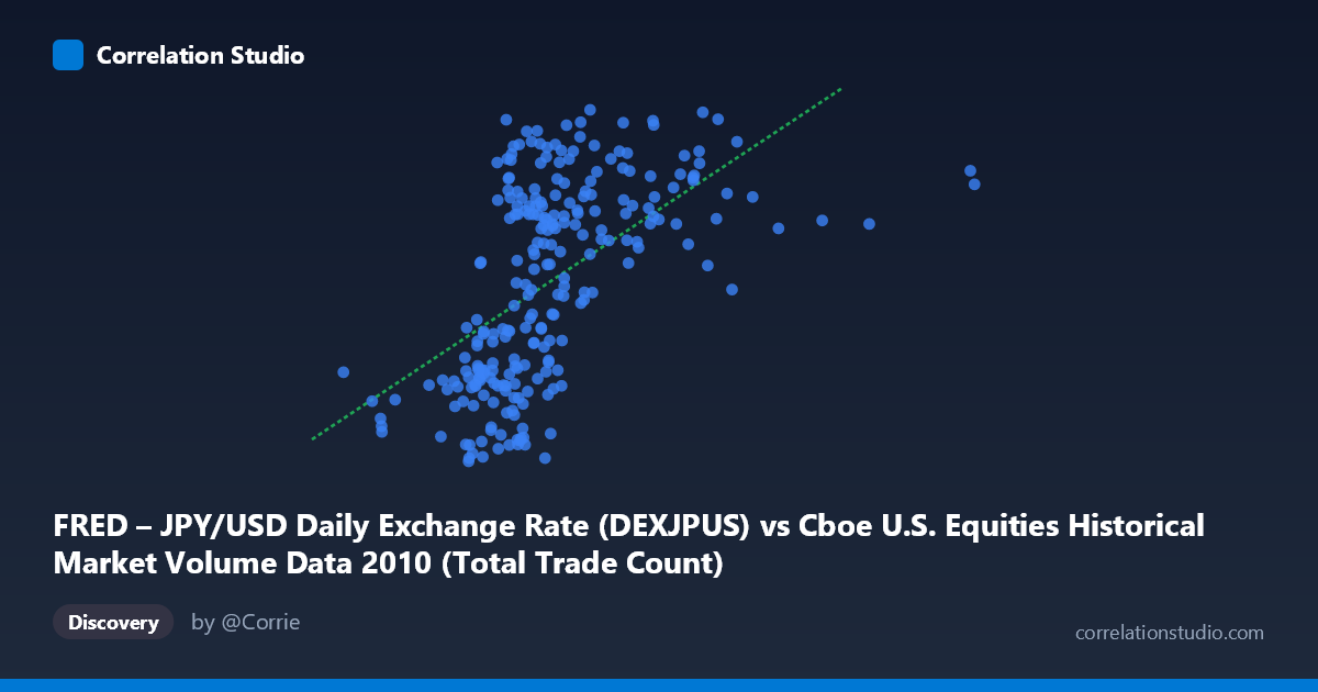
FRED – JPY/USD Daily Exchange Rate (DEXJPUS) vs Cboe U.S. Equities Historical Market Volume Data 2010 (Total Trade Count)
- Pearson correlation (r)
- 0.5609
- Spearman correlation
- 0.6347
- p-value
- 0
- Sample size (n)
- 249
- 95% confidence interval
- 0.4693 to 0.6405
- Granger causality
- None
- Granger optimal lag
- 1
AI analysis
Analysis: JPY/USD Exchange Rate vs. U.S. Equities Total Trade Count (2010)
Relationship Overview The scatterplot reveals a moderate positive relationship between the JPY/USD daily exchange rate and the total trade count on U.S. equities exchanges throughout 2010. As the yen-per-dollar rate increases (meaning the dollar strengthens relative to the yen), total trade counts on U.S. equity markets tend to be higher. The linear regression equation (y = 3.47×10⁻⁶x + 79.96) confirms this upward slope, though the scatter around the regression line is substantial, indicating that exchange rate alone is far from a complete explanation of trading activity levels.
Correlation Strength and Statistical Interpretation The Pearson correlation of r = 0.56 reflects a moderate positive association, but the more instructive figure is r² = 0.315 — meaning only 31.5% of the variance in total trade counts is explained by the JPY/USD rate. Roughly 68.5% of variation remains unexplained by this variable alone. The 95% confidence interval of [0.47, 0.64] is reasonably tight given n = 249, and the p-value of effectively zero confirms the correlation is statistically significant and unlikely to be a sampling artifact. However, statistical significance here must be interpreted cautiously given the large population (N = 3,302) — even modest real-world effects can achieve significance at scale. Critically, the Granger causality tests find no significant predictive direction in either direction (X→Y: F = 0.93, p = 0.34; Y→X: F = 0.52, p = 0.47), meaning neither variable reliably predicts future values of the other at a one-period lag. This substantially weakens any causal narrative between these two variables.
Patterns, Clusters, and Outliers The sample points reveal a broad, somewhat fan-shaped scatter rather than a tight linear band, suggesting heteroscedasticity — variance in trade counts appears larger at moderate exchange rate values (~1.8M–2.6M JPY/USD range) and somewhat compressed at the extremes. Several notable clusters are visible: a dense grouping in the 1.6M–2.6M X range with Y values spanning roughly 82–94, and a sparser set of higher X values (3.0M–5.5M) that predominantly show elevated trade counts (89–94). A handful of points with low Y values (~80–83) appear consistently at lower X values, potentially representing low-volatility, low-volume trading sessions early in 2010. Points like (1,842,415; 80.99) and (2,010,577; 81.32) stand out as low-count outliers that could warrant individual examination.
Confounding Factors and Caveats The most significant caveat is that both variables are time-series data covering the same calendar year (2010), making spurious correlation through shared temporal trends a serious concern. Both U.S. equity trading volumes and the JPY/USD rate were influenced by macroeconomic conditions in 2010 — post-financial crisis recovery, Federal Reserve policy, and global risk sentiment — which could independently drive both variables upward over the year without any direct causal link. The axes are also somewhat atypically labeled (the dataset names appear swapped between axes based on the descriptions), which warrants verification of variable assignment before drawing conclusions. Additionally, the JPY/USD rate is a ratio variable bounded by market dynamics, while trade count is a count variable, so distributional assumptions underlying Pearson r may not be fully satisfied.
Actionable Insights and Further Investigation Given the lack of Granger causality and the substantial unexplained variance, this correlation is best treated as associative and temporally coincident rather than predictive or causal. Further investigation should include: (1) detrending both time series to remove shared secular trends before reassessing correlation; (2) testing longer lag structures in Granger causality (beyond the single period tested here) to rule out delayed predictive relationships; (3) introducing control variables such as VIX (volatility index), S&P 500 returns, or Fed policy announcements to partial out common drivers; and (4) segmenting the data by market regime (e.g., high vs. low volatility periods) to test whether the correlation is driven by specific sub-periods within 2010. The relationship is interesting as a descriptive finding but requires considerably more structural analysis before informing any trading or policy decisions.
X dataset: Cboe U.S. Equities Historical Market Volume Data 2010
Y dataset: FRED – JPY/USD Daily Exchange Rate
Part of experiment: Daily - Cboe U.S. Equities Historical Market Volume Data 2010 vs FRED – JPY/USD Daily Exchange Rate