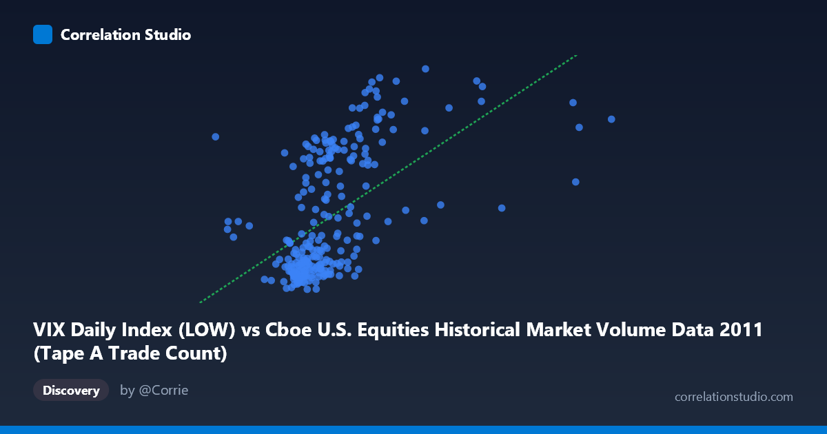
VIX Daily Index (LOW) vs Cboe U.S. Equities Historical Market Volume Data 2011 (Tape A Trade Count)
- Pearson correlation (r)
- 0.5507
- Spearman correlation
- 0.6247
- p-value
- 0
- Sample size (n)
- 252
- 95% confidence interval
- 0.4583 to 0.6313
- Granger causality
- None
- Granger optimal lag
- 1
AI analysis
Scatterplot Analysis: VIX Low vs. Tape A Trade Count (2011)
Relationship Overview
The scatterplot reveals a moderate positive relationship between the VIX Daily Index (Low) and the Tape A Trade Count for U.S. equities in 2011. As the VIX low values increase — indicating elevated baseline fear or uncertainty in the market — trade counts on Tape A tend to rise correspondingly. This aligns intuitively with market microstructure theory: periods of heightened volatility typically spur increased trading activity as participants reposition, hedge, or react to rapidly changing prices. The linear regression equation (y = 1.32369E-05x + 7.3418) suggests a modest but meaningful slope, meaning each unit increase in VIX low is associated with a measurable uptick in trade count.
Correlation Strength and Statistical Significance
The Pearson correlation of r = 0.5507 indicates a moderate positive association, but the explanatory power is more sobering: r² = 0.3033, meaning only about 30.3% of the variance in Tape A Trade Count is explained by VIX Low values. Nearly 70% of the variation remains attributable to other factors. The 95% confidence interval of [0.4583, 0.6313] is meaningfully above zero and relatively tight given the large paired sample (n = 252, N = 3,780), and the p-value of essentially 0 confirms the correlation is highly unlikely to be a statistical artifact. However, statistical significance should not be conflated with practical magnitude — a moderate r in a noisy financial system still leaves substantial unexplained variance. Critically, the Granger causality tests show no significant directional predictive relationship in either direction (X→Y: F = 0.08, p = 0.78; Y→X: F = 0.12, p = 0.73), meaning neither variable reliably forecasts the other at a one-period lag. This severs any straightforward causal or even predictive trading narrative from these data alone.
Notable Patterns, Clusters, and Outliers
The sample points reveal several important structural features. A dense cluster exists in the lower-left region, with VIX Low values roughly between 900,000–1,200,000 and trade counts concentrated below ~22, suggesting a large proportion of "normal" market days with moderate volatility and routine trading volumes. Above a VIX Low threshold of approximately 1,400,000–1,500,000, trade counts begin to accelerate noticeably, with several points exceeding 30–40 — consistent with elevated-stress market episodes during 2011 (e.g., the U.S. debt ceiling crisis and European sovereign debt contagion in mid-to-late summer). A handful of points at extreme X values (e.g., ~2,126,541 paired with a trade count of 37.50, and ~1,876,408 with 24.70) appear as potential outliers that may disproportionately influence the regression slope. The relationship also appears to exhibit some non-linearity, with variance in Y widening considerably at higher X values — a pattern suggestive of heteroscedasticity rather than a clean linear fit.
Confounding Factors and Caveats
Several important caveats temper interpretation. First, both variables may be jointly driven by third-party factors — major macroeconomic announcements, Federal Reserve statements, or geopolitical shocks in 2011 could simultaneously spike VIX and drive trading volumes without one causing the other. Second, the dataset covers a single calendar year (2011), which was anomalously volatile (S&P 500 downgrade, European debt crisis), so the observed correlation may not generalize to other market regimes. Third, the axis labeling appears inverted relative to typical conventions — VIX data appears on the X-axis drawn from a market volume dataset, and trade counts on the Y-axis drawn from a VIX dataset — suggesting a possible data join or labeling artifact that warrants verification. Fourth, heteroscedasticity in the residuals (wider spread at higher VIX values) violates a key assumption of ordinary least squares regression, potentially inflating confidence in the linear fit.
Actionable Insights and Further Investigation
Despite the absence of Granger causality, the moderate correlation and clear clustering pattern offer actionable starting points. Analysts should investigate non-linear model fits (e.g., polynomial or logarithmic regression) to better capture the apparent acceleration in trade count at high VIX levels. Regime segmentation — separating calm periods (VIX Low < 15) from stress periods (VIX Low 25) — could reveal whether the correlation strengthens materially in high-volatility regimes, which would have implications for liquidity provisioning and market-making strategies. Introducing additional covariates such as S&P 500 returns, bid-ask spreads, or options volume could improve the explained variance well beyond the current 30.3%. Finally, extending the analysis across multiple years (2008–2023) would test whether 2011's unusually turbulent conditions are inflating the observed correlation, and whether any regime-dependent Granger causality emerges at lags beyond one period.
X dataset: Cboe U.S. Equities Historical Market Volume Data 2011
Y dataset: VIX Daily Index
Part of experiment: Daily - Cboe U.S. Equities Historical Market Volume Data 2011 vs VIX Daily Index