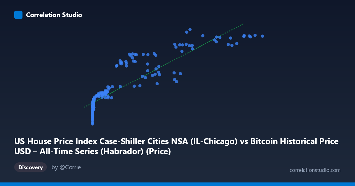
US House Price Index Case-Shiller Cities NSA (IL-Chicago) vs Bitcoin Historical Price USD – All-Time Series (Habrador) (Price)
- Pearson correlation (r)
- 0.8883
- Spearman correlation
- 0.9626
- p-value
- 0
- Sample size (n)
- 187
- 95% confidence interval
- 0.8536 to 0.9152
- Granger causality
- None
- Granger optimal lag
- 1
AI analysis
Analysis: Bitcoin Price vs. Chicago Case-Shiller Home Price Index
1. What the Visualization Reveals
The scatterplot shows a strong positive but distinctly non-linear relationship between Bitcoin's USD price (X-axis) and the Chicago Case-Shiller Home Price Index (Y-axis). Given Bitcoin's price spans nearly six orders of magnitude (0.06 to 118,670), while the housing index moves in a comparatively narrow band (102.75 to 223.75), the data exhibits a classic logarithmic/saturating curve shape: Y rises steeply as X moves from near-zero into the hundreds, then the rate of increase flattens considerably as X climbs into the tens of thousands. A linear fit still captures a large share of variance, but this is largely an artifact of both series trending upward together over the same time period.
2. Strength, Direction, and Statistical Caveats
The correlation coefficient (r = 0.888, R² = 0.789) indicates that a linear model explains roughly 79% of the variance in Y from X — a strong statistical association. The 95% CI [0.854, 0.915] is tight and the p-value is effectively 0, meaning the correlation is highly unlikely to be due to sampling noise. However, statistical significance here should not be confused with a causal or economically meaningful relationship. The Granger causality tests show no significant predictive direction in either direction (X→Y: p=0.32; Y→X: p=0.18), meaning neither series' past values help forecast the other's future values once autocorrelation is accounted for. This is a critical finding: it strongly suggests the correlation is driven by both variables independently trending upward over the 2010–2026 window (i.e., a shared time trend), rather than one asset influencing the other.
3. Notable Patterns and Outliers
Several features stand out: - Compression at low X values: Hundreds of early Bitcoin prices (sub-$1000) correspond to Y values clustered tightly between ~103–140, showing housing prices barely moved while Bitcoin was still negligible in value. - Divergence/scatter at high X: At X 50,000, Y values range widely (157 to 224) for similar X levels (e.g., X≈57,000 gives Y=172 in one instance and Y=211 in another), indicating the relationship weakens or becomes noisy at scale — likely reflecting Bitcoin's extreme volatility (crashes/rallies) occurring within periods of steadily rising home prices. - Curve, not line: The steep early rise followed by flattening is consistent with a log-linear relationship (Y vs. log(X)) rather than the linear fit provided, which may understate fit quality in the low-X region and overstate it in the high-X region.
4. Confounding Factors and Caveats
This is very likely a spurious correlation driven by time rather than a genuine economic relationship. Both Bitcoin price and the Chicago housing index have risen substantially from 2010–2026 due to entirely different macro drivers: housing prices respond to mortgage rates, local supply/demand, and broad inflation, while Bitcoin is driven by speculative demand, adoption cycles, and crypto-specific events (halvings, exchange collapses, regulatory news). Since both are non-stationary trending time series, any two upward-trending series over the same period will show artificially high correlation — a well-known statistical pitfall. The lack of Granger causality reinforces that this is a coincidental co-trending pattern, not a predictive or mechanistic link.
5. Suggestions for Further Investigation
- Test for spurious regression: Run a cointegration test (e.g., Engle-Granger) to check if these series share a genuine long-run equilibrium, or difference both series (e.g., % change month-over-month) and re-run correlation — this should collapse dramatically if the relationship is merely trend-driven. - Control for a common macro factor: Introduce a third variable like CPI/inflation, M2 money supply, or interest rates, which likely drive both series independently — a partial correlation controlling for these would clarify true relationship strength. - Re-fit with log(X): Given the visual curvature, a log-linear or log-log model would likely produce a better-specified fit than the current linear equation, especially for interpreting the low-X cluster. - Practical takeaway: Despite the high R², this pairing should not be used for forecasting one asset from the other — the Granger results confirm no exploitable lead-lag relationship exists for trading or planning purposes.
X dataset: Bitcoin Historical Price USD – All-Time Series (Habrador)
Y dataset: US House Price Index Case-Shiller Cities NSA
Part of experiment: Bitcoin - Bitcoin Historical Price USD – All-Time Series (Habrador) vs US House Price Index Case-Shiller Cities NSA