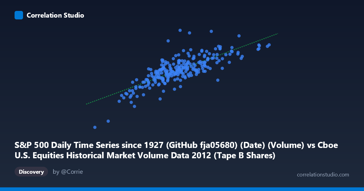
S&P 500 Daily Time Series since 1927 (GitHub fja05680) (Date) (Volume) vs Cboe U.S. Equities Historical Market Volume Data 2012 (Tape B Shares)
- Pearson correlation (r)
- 0.7813
- Spearman correlation
- 0.7699
- p-value
- 0
- Sample size (n)
- 250
- 95% confidence interval
- 0.7278 to 0.8254
- Granger causality
- None
- Granger optimal lag
- 10
AI analysis
Analysis: S&P 500 Daily Volume vs. Cboe Tape B Shares (2012)
Relationship Overview The scatterplot reveals a moderately strong positive linear relationship between total U.S. equity market volume (X-axis, sourced from the S&P 500 daily time series dataset) and Cboe Tape B share volume (Y-axis, from the Cboe historical market volume data) across 250 trading days in 2012. As overall market volume increases, Tape B shares traded tend to rise proportionally, which is intuitively sensible — Tape B covers NYSE American (AMEX)-listed securities, and its trading activity would naturally expand and contract alongside broader market participation. The linear regression equation y = 29.751x + 1.544B suggests that for every additional share of total market volume, Tape B volume increases by approximately 29.75 shares, with a substantial baseline intercept reflecting the minimum structural activity in this market segment.
Correlation Strength and Statistical Significance The Pearson correlation of r = 0.7813 indicates a strong positive association, and the R² of 0.6105 means that approximately 61% of the variance in Tape B share volume is explained by total market volume — a meaningful but incomplete explanation, leaving roughly 39% attributable to other factors. The 95% confidence interval for r of [0.7278, 0.8254] is relatively narrow given the sample size of n = 250 (drawn from a population of N = 3,750), and the p-value of effectively 0 confirms this relationship is highly statistically significant and not a chance finding. However, the Granger causality results complicate the narrative considerably: neither direction (X→Y nor Y→X) shows significant temporal predictive power at the optimal 10-period lag (F = 1.41, p = 0.177 for X→Y; F = 0.77, p = 0.662 for Y→X). This means that while the two series are strongly correlated contemporaneously, knowing past values of one does not help forecast the other — they move together but neither leads the other in time.
Patterns, Clusters, and Outliers The scatterplot exhibits a fairly coherent linear cloud, though with notable spread that widens at higher volume levels, suggesting mild heteroscedasticity. Several prominent outliers are visible: one point near (70.6M, 5.27B) stands dramatically above the regression line, representing an anomalous day where Tape B volume surged far beyond what total market volume would predict. Another cluster of points in the lower-left quadrant (X: ~40–55M, Y: ~2.5–3.2B) corresponds to low-volume trading days — likely holiday-shortened sessions or summer lull periods common in 2012. The upper-right region shows elevated activity around key market events, with points near (110.6M, 4.48B) and (100.8M, 5.04B) standing out as high-volume days, possibly linked to options expiration, Fed announcements, or macro volatility events during 2012 (e.g., the fiscal cliff negotiations).
Confounding Factors and Caveats Several important caveats apply to this analysis. First, the dataset labeling appears cross-referenced — the X-axis column is described as "Volume" from the S&P 500 time series dataset, while the Y-axis is "Tape B Shares" from the Cboe dataset, suggesting these may be joined on date rather than being structurally independent measurements, which inflates the apparent meaningfulness of the correlation. Second, both series are subject to common market-wide drivers — volatility regimes, institutional rebalancing, index reconstitution events, and algorithmic trading patterns — which act as latent confounders that could independently elevate both measures simultaneously. Third, the single-year scope (2012 only) limits generalizability; market microstructure, exchange competition, and Tape B composition may behave differently across different market regimes.
Actionable Insights and Further Investigation Practitioners interested in using total market volume as a proxy or predictor for Tape B activity should note that while the contemporaneous relationship is strong, the lack of Granger causality means intraday or lagged forecasting models built on this relationship alone would likely underperform. Further investigation should include: (1) extending the time series beyond 2012 to test whether this correlation is stable across different volatility regimes; (2) decomposing the 39% unexplained variance by examining Tape B-specific drivers such as AMEX-listed ETF activity or sector-specific events; (3) testing shorter lags (1–3 days) in Granger tests, as the 10-period optimal lag may obscure short-term predictive signals; and (4) investigating the extreme outlier at ~5.27B Tape B shares to identify the specific date and market event, as it may represent a data quality issue or a genuinely significant structural episode worth understanding in isolation.
X dataset: Cboe U.S. Equities Historical Market Volume Data 2012
Y dataset: S&P 500 Daily Time Series since 1927 (GitHub fja05680) (Date)
Part of experiment: Daily - Cboe U.S. Equities Historical Market Volume Data 2012 vs S&P 500 Daily Time Series since 1927 (GitHub fja05680) (Date)