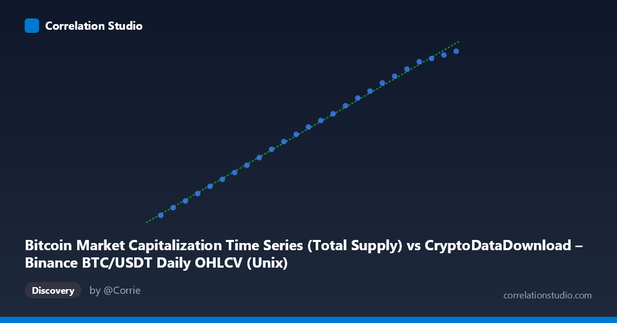
Bitcoin Market Capitalization Time Series (Total Supply) vs CryptoDataDownload – Binance BTC/USDT Daily OHLCV (Unix)
- Pearson correlation (r)
- 0.9989
- Spearman correlation
- 1
- p-value
- 0
- Sample size (n)
- 25
- 95% confidence interval
- 0.9975 to 0.9995
- Granger causality
- None
- Granger optimal lag
- 6
AI analysis
Analysis: Bitcoin Market Cap Time Series vs. Circulating Supply (Time-Indexed)
1. What the Visualization Reveals
The scatterplot shows an extremely tight, near-perfect linear relationship between the two variables across the 25-day observation window (March 29 – April 22, 2024). Both series increase monotonically with time, and when plotted against each other they form a virtually unbroken straight line with almost no scatter around the regression trend. This is a textbook example of two variables that are both strongly trending in the same direction over a short time window.
2. Strength, Direction, and Predictive Relationship
The correlation is essentially maximal (r = 0.9989, r² = 0.9978), meaning that 99.78% of the variance in Y is statistically explained by X under a simple linear model. The 95% confidence interval [0.9975, 0.9995] is extremely narrow and does not approach zero, and the p-value is effectively 0 — so the linear association is not a artifact of sampling noise; it is a robust feature of this dataset. In practical terms, knowing X allows near-perfect prediction of Y across this range.
However, the Granger causality tests tell a different story about temporal dynamics: neither X→Y (F=0.858, p=0.572) nor Y→X (F=0.851, p=0.575) is significant at any conventional threshold. This means that past values of one series do not help predict future changes in the other beyond what the series' own history already provides. The strong contemporaneous correlation is not evidence of one variable driving or leading the other in time — it reflects that both variables are independently and smoothly trending upward over the same short window, not a genuine lead-lag causal relationship.
3. Notable Patterns and Features
- The relationship is smoothly monotonic with no visible outliers, clusters, or regime breaks — every point lies close to the regression line. - There is a subtle hint of mild curvature (slightly steeper slope in the later dates) consistent with BTC's price acceleration in early April 2024, but the deviation from linearity is small enough that a linear fit still captures ~99.8% of variance. - No cyclical, seasonal, or discontinuous jumps are apparent — consistent with a short, trending market period rather than a full price cycle.
4. Confounding Factors and Caveats
This is a classic case of spurious/trend-driven correlation risk: both series are time-indexed and monotonically increasing over just 25 days, and any two smoothly trending series over a short window will show high r² purely due to shared trend with time, not necessarily due to a real economic linkage. Specific caveats: - Autocorrelation: Both series are highly autocorrelated (each day resembles the prior day), inflating the apparent correlation and reducing effective degrees of freedom — the "N=25" independent observations assumption is likely violated. - Definitional overlap: Market cap is mechanically derived from price × circulating supply; if Y is closely tied to circulating supply (which grows almost linearly via mining issuance) while X reflects price/market cap, part of the "relationship" may be a mathematical artifact of how these metrics are constructed rather than an economically meaningful signal. - Short window: 25 days is too short to assess long-run causality, structural breaks, or regime changes (e.g., halving effects, since this period is just before the April 2024 Bitcoin halving).
5. Suggested Further Investigation
- Detrend or difference both series (e.g., first differences or % daily change) and re-run correlation/Granger tests to check whether the relationship holds beyond shared trend — this is essential given the non-significant Granger results despite high r². - Extend the time window to include more volatile/non-trending periods (e.g., post-halving, or a bear market phase) to test whether the relationship is stable or specific to this trending regime. - Clarify variable construction: confirm whether Y is truly independent of X (e.g., circulating supply vs. derived market cap) to rule out definitional double-counting. - Given the lack of Granger causality, treat this relationship as descriptive/correlational only — not suitable for forecasting one series from lagged values of the other without further validation on differenced or detrended data.
X dataset: CryptoDataDownload – Binance BTC/USDT Daily OHLCV
Y dataset: Bitcoin Market Capitalization Time Series
Part of experiment: Bitcoin - CryptoDataDownload – Binance BTC/USDT Daily OHLCV vs Bitcoin Market Capitalization Time Series