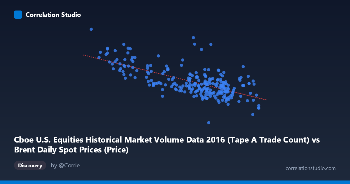
Cboe U.S. Equities Historical Market Volume Data 2016 (Tape A Trade Count) vs Brent Daily Spot Prices (Price)
- Pearson correlation (r)
- -0.6729
- Spearman correlation
- -0.6012
- p-value
- 0
- Sample size (n)
- 251
- 95% confidence interval
- -0.7354 to -0.599
- Granger causality
- None
- Granger optimal lag
- 10
AI analysis
Analysis: Brent Crude Oil Prices vs. Cboe U.S. Equities Trade Count (2016)
Relationship Overview The scatterplot reveals a moderately strong negative relationship between Cboe U.S. equities trade count (Tape A) and Brent crude oil spot prices across 2016. As equity market trade volume increases, Brent crude prices tend to decrease — and conversely, lower trade activity coincides with higher oil prices. The linear regression equation (y = -29,755.5x + 2,690,680) quantifies this: each additional unit increase in trade count is associated with a ~$29,755 decline in the Brent price index. The data spans a meaningful range — trade counts from ~26 to ~55 units and Brent prices from ~$540K to ~$2.5M in the scaled units provided — suggesting this is not a trivially narrow relationship.
Correlation Strength and Statistical Significance The correlation of r = -0.6729 is moderate-to-strong, and the r² of 0.4528 indicates that approximately 45.3% of the variance in Brent crude prices is statistically explained by equity trade count variation. While this is a substantial share, it equally means ~55% of variance remains unexplained by this single variable. The 95% confidence interval of [-0.7354, -0.5990] is relatively tight and does not cross zero, and the p-value of effectively 0 confirms the correlation is highly statistically significant in this sample. However, the Granger causality tests tell a critical story: neither direction (X→Y nor Y→X) reaches significance (F ≈ 0.75, p ≈ 0.67 for both), even at an optimal lag of 10 periods. This means that neither variable temporally predicts the other — the correlation, however strong in cross-sectional terms, does not imply a leading/lagging predictive relationship useful for forecasting.
Notable Patterns and Outliers Several features stand out in the sample data. There is a visible cluster of points in the mid-range (trade counts ~44–50, prices ~$1.1M–$1.5M), suggesting a dense "core" regime for 2016 market conditions. At the lower end of the trade count axis (26–34 range), prices are consistently elevated ($1.7M–$2.5M), which may correspond to low-volatility or holiday-thinned trading days when oil prices were also relatively higher (early-to-mid 2016 recovery period). The point at (26.01, 2,497,318) is a notable high-leverage outlier that likely exerts disproportionate influence on the regression slope. At the upper trade-count extreme (~53), prices dip toward ~$1.0M, consistent with high-activity, risk-on equity sessions coinciding with lower oil prices later in 2016.
Confounding Factors and Caveats The most significant caveat is the dataset mismatch implied by the column labels: the X-axis (trade count) is listed as coming from the "Brent Daily Spot Prices" dataset, and the Y-axis (Brent price) from the "Cboe volume" dataset — suggesting a data join or file labeling inconsistency that warrants verification. More substantively, both variables are likely driven by shared macro factors in 2016 — particularly the oil price recovery from January lows, Brexit volatility in June, and the post-U.S. election rally in November/December — meaning the correlation may largely reflect parallel responses to common economic shocks rather than any direct relationship. Seasonal patterns in equity trading volume (e.g., lower volume in summer and around holidays) may also confound the signal, as these same periods could coincide with distinct oil price regimes.
Actionable Insights and Further Investigation Given the absence of Granger causality, practitioners should not use equity trade count as a leading indicator for Brent prices or vice versa in any trading or forecasting model. However, the shared explained variance (~45%) makes this relationship worth investigating as a proxy for a common latent factor — likely broader market risk appetite or macro uncertainty. Recommended next steps include: (1) introducing explicit control variables such as USD index, S&P 500 returns, or VIX to test whether the correlation disappears after controlling for macro risk; (2) segmenting the time series by known 2016 macro regimes (pre/post-Brexit, pre/post-election) to test whether the correlation is stable or regime-dependent; and (3) verifying the dataset join to ensure trade count and price observations are correctly aligned by date before drawing further conclusions.
X dataset: Brent Daily Spot Prices
Y dataset: Cboe U.S. Equities Historical Market Volume Data 2016
Part of experiment: Daily - Brent Daily Spot Prices vs Cboe U.S. Equities Historical Market Volume Data 2016