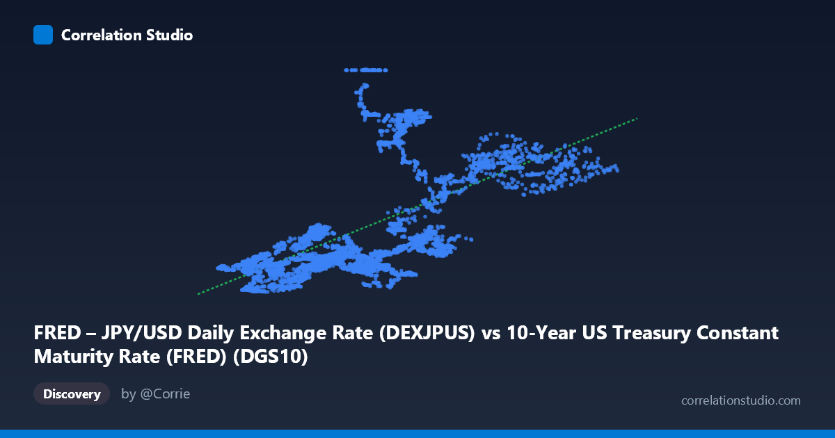
FRED – JPY/USD Daily Exchange Rate (DEXJPUS) vs 10-Year US Treasury Constant Maturity Rate (FRED) (DGS10)
- Pearson correlation (r)
- 0.6066
- Spearman correlation
- 0.6809
- p-value
- 0
- Sample size (n)
- 13815
- 95% confidence interval
- 0.596 to 0.617
- Granger causality
- None
- Granger optimal lag
- 1
AI analysis
Analysis: JPY/USD Exchange Rate vs. 10-Year US Treasury Yield
1. Overall Relationship The scatterplot reveals a moderate positive relationship between the JPY/USD exchange rate (yen per dollar) and the 10-Year US Treasury constant maturity yield. As the dollar strengthens against the yen (higher JPY/USD values), Treasury yields tend to be higher. The linear regression equation (y = 13.40x + 75.99) suggests that each additional yen per dollar is associated with roughly 13.4 basis points of additional yield. However, the scatter around this trend line is substantial, and several distinct clusters and outliers are immediately visible, indicating that the relationship is far from deterministic and likely reflects shared macroeconomic regimes rather than a direct causal link.
2. Correlation Strength and Statistical Framing The Pearson correlation of r = 0.607 is statistically significant (p ≈ 0, N = 13,815), but the more informative figure is R² = 0.368 — meaning only 36.8% of the variance in Treasury yields is explained by the exchange rate. Nearly two-thirds of yield variation is attributable to other factors entirely. The 95% confidence interval [0.596, 0.617] is narrow given the large sample, confirming the correlation estimate is precise, but precision does not imply practical sufficiency. Critically, the Granger causality tests find no significant predictive direction in either direction (X→Y: F=0.79, p=0.37; Y→X: F=3.52, p=0.06). Neither variable reliably predicts the other at a one-period lag, reinforcing that this correlation is likely a spurious co-movement driven by shared underlying macro drivers rather than any mechanistic transmission between exchange rates and yields.
3. Notable Patterns, Clusters, and Outliers The sample points reveal several striking structural features. There is a dense cluster of observations at relatively low X values (~1–5 JPY/USD range is absent given the actual range starts at ~75–160 yen), with most Y values (yields) concentrated in the 100–200 basis point range, suggesting extended periods of low-rate, strong-yen environments (post-2008 era). A second, clearly identifiable cluster appears at Y values near 357–358, visible in multiple sample points (e.g., 6.11→357.56, 6.62→357.40, 6.66→357.46), forming a nearly horizontal band that suggests a data artifact, regime ceiling, or capped measurement worth investigating. Additionally, outlier points like (1.99, 80.21) and (3.17, 80.66) sit at the low extreme, while (14.11, 215.78) and (10.50, 249.00) sit at the upper right, consistent with early-1980s or mid-cycle high-yield, weak-yen periods. These clusters suggest the data encodes distinct historical regimes rather than a smooth continuous relationship.
4. Confounding Factors and Caveats Several confounds make causal interpretation problematic. Both variables are heavily trend-driven time series spanning 1971–2026, meaning they share common macro epoch structures: the high-inflation 1970s–80s, the post-Plaza Accord yen appreciation, the post-2008 zero-lower-bound era, and post-2022 divergence. This creates spurious correlation from shared temporal trends rather than structural linkage. The Bank of Japan's ultra-loose monetary policy (yield curve control) and the Federal Reserve's rate cycles have driven both variables simultaneously but through separate institutional channels. Furthermore, the suspicious cluster near Y≈357–358 may represent data quality issues — a repeated value, a measurement artifact, or a merged dataset join error — that artificially inflates or distorts the correlation estimate. The axis label swap noted in the metadata (each dataset column appears to be assigned to the opposite axis label) should also be verified before drawing any conclusions.
5. Actionable Insights and Further Investigation Given the lack of Granger causality and the regime-dependent clustering, several follow-up steps are warranted. First, investigate the Y≈357–358 cluster immediately — these repeated values are anomalous and may indicate a data pipeline error in the dataset merge. Second, consider segmenting the analysis by macroeconomic regime (e.g., pre/post-Plaza Accord 1985, pre/post-GFC 2008, pre/post-Fed liftoff 2022) to determine whether the correlation holds within regimes or is purely an artifact of long-run co-trending. Third, apply cointegration testing (e.g., Engle-Granger) to properly assess whether any long-run equilibrium relationship exists between these non-stationary series. Fourth, verify and correct the axis/dataset label assignment, as the metadata suggests columns may be swapped. Finally, incorporating interest rate differentials (US vs. Japan 10-year spread) and intervention episode flags (BOJ FX interventions) as controls would help isolate any genuine exchange rate–yield relationship from institutional noise.
X dataset: 10-Year US Treasury Constant Maturity Rate (FRED)
Y dataset: FRED – JPY/USD Daily Exchange Rate
Part of experiment: Daily - 10-Year US Treasury Constant Maturity Rate (FRED) vs FRED – JPY/USD Daily Exchange Rate