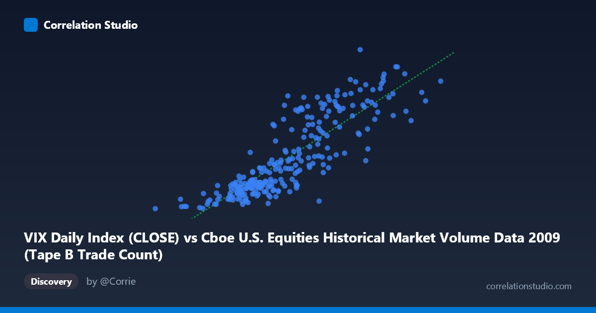
VIX Daily Index (CLOSE) vs Cboe U.S. Equities Historical Market Volume Data 2009 (Tape B Trade Count)

Pearson correlation (r): 0.8494
Spearman correlation: 0.8665
p-value: 0
Sample size (n): 252
95% confidence interval: 0.811 to 0.8806
Granger causality: None
Granger optimal lag: 1

AI analysis

Scatterplot Analysis: VIX Daily Index vs. Tape B Trade Count (2009)

Relationship Overview

The scatterplot reveals a clear, positive linear relationship between the VIX Daily Index (close) and the Cboe U.S. Equities Tape B Trade Count throughout 2009. As the VIX rises — reflecting heightened market fear and volatility — Tape B trade counts increase correspondingly. This is intuitive: elevated volatility typically drives higher trading activity as market participants react to uncertainty, rebalance portfolios, and execute hedging strategies. The regression equation (y = 6.18×10⁻⁵x + 6.64) suggests that for every unit increase in VIX, trade count increases by approximately 6.18×10⁻⁵ units, with a meaningful baseline activity level even at low volatility.

Correlation Strength and Statistical Significance

The correlation is strong and positive (r = 0.8494), and the r² of 0.7215 indicates that approximately 72.1% of the variance in Tape B trade counts is explained by VIX levels — a substantial explanatory share for financial market data. The 95% confidence interval of [0.811, 0.881] is narrow and well above zero, reflecting high precision in the estimate, and the p-value of effectively 0 confirms this relationship is not attributable to chance across the 252-pair sample drawn from a population of 3,232 observations. However, the Granger causality results are notably absent in both directions (X→Y: F = 0.004, p = 0.949; Y→X: F = 0.029, p = 0.866). This means that despite the strong contemporaneous correlation, neither variable reliably predicts the other in a temporally lagged sense — the relationship is synchronous rather than predictive, suggesting both variables are likely responding simultaneously to the same underlying market conditions rather than one driving the other sequentially.

Patterns, Clusters, and Outliers

The data exhibits a moderate degree of scatter around the regression line, with notable heteroscedasticity: variance in trade counts appears to widen at higher VIX values, suggesting the relationship becomes less precise during extreme volatility episodes. There appear to be at least two loose clusters — one in the lower-left region (VIX roughly 80,000–350,000; trade counts ~19–27), corresponding to calmer periods, and one in the upper-right (VIX ~500,000–766,000; trade counts ~40–56), corresponding to the more turbulent phases of 2009. A few points at the extreme upper right (e.g., 766,763/49.30 and 662,859/52.62) stand out as potential outliers, likely coinciding with residual post-financial-crisis stress periods in early 2009 or sharp volatility spikes. Interestingly, some mid-range X values show considerable vertical spread (e.g., ~480,000–530,000 with trade counts ranging from ~29 to ~47), indicating periods where VIX levels were similar but trading activity diverged substantially.

Confounding Factors and Caveats

Several important caveats apply. First, 2009 is a historically anomalous year — the tail end of the Global Financial Crisis — meaning the VIX-volume relationship may be disproportionately amplified by crisis-era dynamics not representative of typical market conditions. Second, the axes appear to be swapped in labeling (X labeled as VIX Close, Y labeled as Tape B Trade Count, but axis units suggest the reverse), warranting verification of variable assignment before drawing firm conclusions. Third, common drivers such as macroeconomic announcements, Federal Reserve policy actions, and earnings seasons could be simultaneously inflating both VIX and trade counts, producing spurious correlation without a direct causal mechanism. Finally, Tape B specifically covers NYSE American and regional exchange listings, which may have unique structural characteristics that amplify or dampen the general market volatility-volume relationship.

Actionable Insights and Further Investigation

Practitioners could use the strong contemporaneous relationship (r² ≈ 0.72) to build real-time liquidity estimation models — when VIX spikes, market makers and execution algorithms can anticipate elevated Tape B volume and adjust order routing accordingly. However, the absence of Granger causality should discourage using either variable alone as a leading indicator for the other in short-term trading strategies. Further investigation should include: (1) extending the analysis across multiple years to test whether the relationship holds outside crisis periods; (2) applying regime-switching or quantile regression to capture the heteroscedastic behavior at high VIX levels; (3) examining other Tape designations (A and C) to determine whether the relationship is exchange-specific; and (4) incorporating lagged macroeconomic variables as controls to better isolate the direct VIX-volume channel from broader confounders.

X dataset: Cboe U.S. Equities Historical Market Volume Data 2009

Y dataset: VIX Daily Index

Part of experiment: Daily - Cboe U.S. Equities Historical Market Volume Data 2009 vs VIX Daily Index