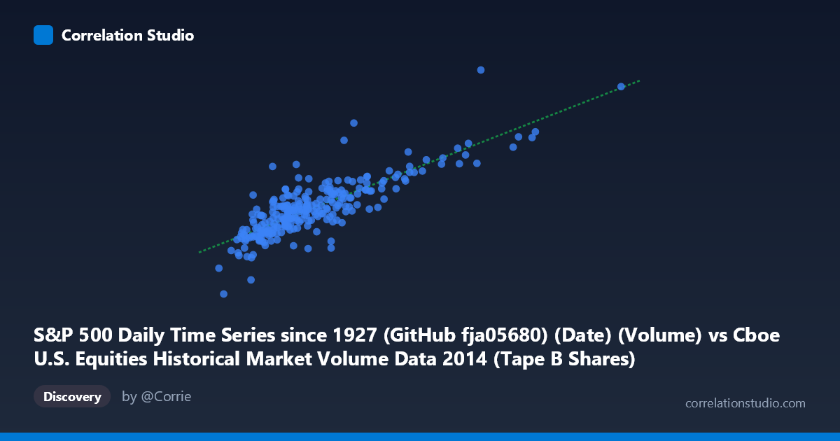
S&P 500 Daily Time Series since 1927 (GitHub fja05680) (Date) (Volume) vs Cboe U.S. Equities Historical Market Volume Data 2014 (Tape B Shares)
- Pearson correlation (r)
- 0.8267
- Spearman correlation
- 0.7845
- p-value
- 0
- Sample size (n)
- 252
- 95% confidence interval
- 0.7832 to 0.8622
- Granger causality
- None
- Granger optimal lag
- 10
AI analysis
Analysis: S&P 500 Daily Volume vs. Cboe Tape B Shares (2014)
Relationship Overview The scatterplot reveals a moderately strong positive relationship between total U.S. equity market volume (X-axis, measured in shares traded across all exchanges and TRFs) and Cboe Tape B shares specifically (Y-axis). As overall market volume rises, Tape B share volume increases correspondingly, which is broadly intuitive — Tape B securities (primarily NYSE American/AMEX-listed stocks and regional exchange issues) tend to participate in broader market-wide volume surges driven by macroeconomic events, volatility spikes, or institutional activity. The linear regression line (y = 22.39x + 1.670B) captures the central tendency reasonably well, though visible scatter around the line suggests meaningful unexplained variation, particularly at higher volume levels where the cloud widens noticeably.
Correlation Strength and Statistical Reliability The Pearson correlation of r = 0.827 indicates a strong positive association, and the R² of 0.683 means that approximately 68.3% of the variance in Tape B shares is explained by total market volume — a substantial but incomplete share, leaving roughly 31.7% attributable to other factors. The 95% confidence interval of [0.783, 0.862] is relatively tight given the sample size of n = 252 trading days, and the p-value of effectively zero confirms this relationship is highly statistically significant and unlikely to be a sampling artifact across the N = 3,686 population context. However, the Granger causality results are notably absent of significance in either direction (X→Y: F = 1.37, p = 0.19; Y→X: F = 0.85, p = 0.58), meaning that neither series reliably predicts the other at a 10-period lag. This is a critical caveat: the two variables move together contemporaneously, but neither leads the other in a temporally predictive sense, suggesting they are co-driven by common market forces rather than one causing the other.
Patterns, Clusters, and Outliers The data exhibits a clear linear core cluster concentrated roughly between 50M–90M total shares (X) and 2.5B–4.0B Tape B shares (Y), representing typical low-to-moderate volatility trading days in 2014. Several notable outliers appear in the upper-right region — points near X = 155M–165M paired with Y values approaching 5.0B–5.1B — which likely correspond to specific high-volatility events such as geopolitical shocks (Russia/Ukraine tensions, October 2014 market correction) or Federal Reserve announcement days. One point near (50.96M, 1.735B) stands out as a low-volume outlier well below the regression line, possibly a holiday-shortened session or data anomaly. The scatter also widens heteroscedastically at higher X values, suggesting the relationship becomes less predictable during extreme volume days.
Confounding Factors and Interpretation Caveats Several confounding factors limit causal interpretation. First, both variables are driven by the same underlying market-wide liquidity conditions — VIX spikes, earnings seasons, and macro announcements simultaneously inflate all tape volumes, creating spurious correlation independent of any Tape B-specific dynamic. Second, market structure changes in 2014 (exchange fee adjustments, maker-taker rule debates, fragmentation shifts) could alter the Tape B share of total volume independently of aggregate volume levels. Third, the X-axis label metadata appears inconsistent — it references "S&P 500 Volume" from one dataset but represents total U.S. equity market volume from Cboe data, suggesting a potential data join mismatch that warrants verification. Finally, 2014 is a single calendar year, limiting generalizability across different market regimes.
Actionable Insights and Further Investigation Practitioners should not treat this correlation as predictive in isolation, given the failed Granger causality tests — real-time forecasting models using lagged total volume to predict Tape B shares would likely underperform. A more productive investigation would decompose residuals to identify which specific days deviate most from the regression line, potentially revealing Tape B-specific structural patterns (e.g., sector rotations into AMEX-listed ETFs or small-caps). It would also be valuable to segment by market volatility regime (using VIX quartiles) to test whether the correlation strengthens during high-volatility periods, which the heteroscedastic scatter hints at strongly. Finally, extending the analysis across multiple years (2010–2023) would test whether this relationship is stable or regime-dependent, particularly around post-2020 retail trading surges that dramatically reshaped tape composition dynamics.
X dataset: Cboe U.S. Equities Historical Market Volume Data 2014
Y dataset: S&P 500 Daily Time Series since 1927 (GitHub fja05680) (Date)
Part of experiment: Daily - Cboe U.S. Equities Historical Market Volume Data 2014 vs S&P 500 Daily Time Series since 1927 (GitHub fja05680) (Date)