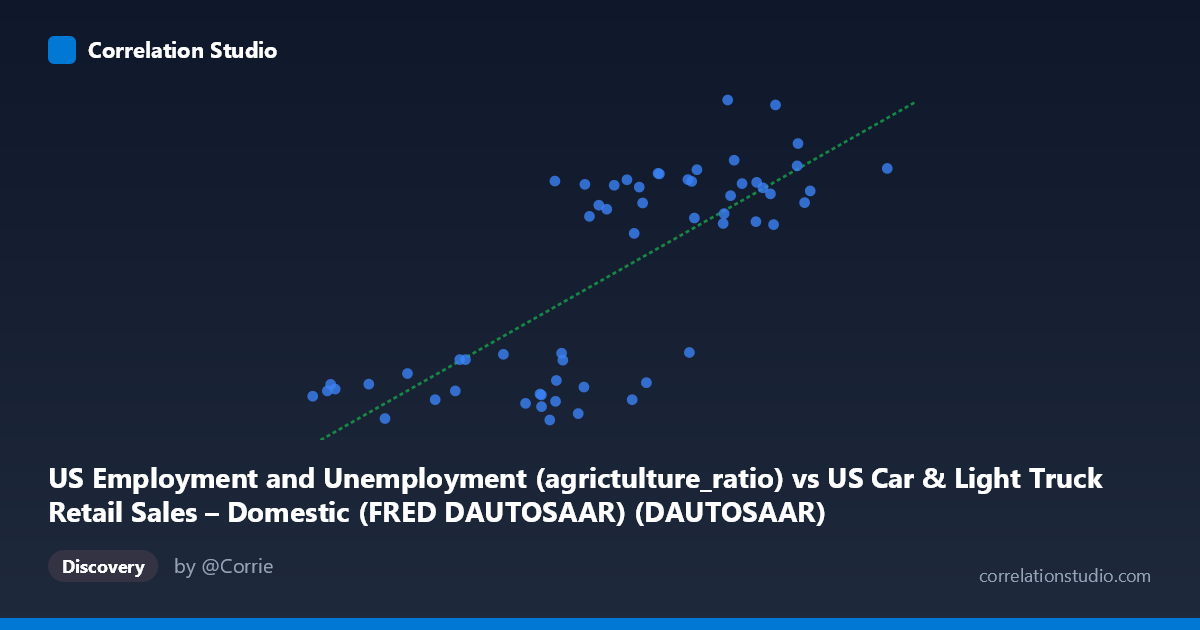
US Employment and Unemployment (agrictulture_ratio) vs US Car & Light Truck Retail Sales – Domestic (FRED DAUTOSAAR) (DAUTOSAAR)
- Pearson correlation (r)
- 0.7634
- Spearman correlation
- 0.7373
- p-value
- 0
- Sample size (n)
- 59
- 95% confidence interval
- 0.6306 to 0.8528
- Granger causality
- None
- Granger optimal lag
- 10
- Time coverage
- 1967-01-01 to 2025-01-01
- Recomputed on refreshed data
- 2026-10-20 (r was 0.7634)
AI analysis
Analysis: US Agriculture Employment Ratio vs. Domestic Auto Retail Sales
1. Overall Relationship The scatterplot reveals a moderate-to-strong positive relationship between the US agriculture employment ratio (X) and domestic auto retail sales (Y). As the agriculture ratio increases from roughly 1.86 to 10.14, auto sales trend upward from approximately 2,095 to 3,844 units (SAAR). The linear regression equation — y = 215.55x + 1,560.45 — implies that for each one-unit increase in the agriculture ratio, auto sales increase by roughly 216 units on an annualized basis. While the upward trend is clearly visible, the data cloud shows considerable vertical scatter at every X value, signaling that the relationship, though real, is far from deterministic.
2. Correlation Strength and Statistical Significance The Pearson correlation of r = 0.763 indicates a meaningfully positive association, but the more policy-relevant figure is R² = 0.583: only about 58% of the variance in auto sales is explained by the agriculture employment ratio, leaving 42% attributable to other factors. The 95% confidence interval for r of [0.631, 0.853] is reassuringly narrow and sits well above zero, and the p-value of 2.07 × 10⁻¹² confirms the association is highly statistically significant across the 59 paired observations drawn from an 86-point population spanning 1967–2025. Crucially, however, Granger causality testing finds no significant predictive direction in either direction (X→Y: F = 1.31, p = 0.274; Y→X: F = 0.93, p = 0.524), even at an optimal lag of 10 periods. This means that while the two series move together, neither reliably leads the other in a temporally predictive sense — the correlation should not be interpreted as evidence of a causal mechanism.
3. Notable Patterns, Clusters, and Outliers The data exhibits a visible bimodal clustering structure: a dense lower-left cluster (X ≈ 1.86–5.5, Y ≈ 2,095–2,460) and a upper-right cluster (X ≈ 7.5–10.14, Y ≈ 3,163–3,844), with a relatively sparse middle zone. This gap may reflect distinct economic regimes or structural breaks across the 58-year time span. Several notable outliers deserve attention: (8.53, 3,817) and (7.84, 3,844) sit well above the regression line, while (7.29, 2,464) and (6.46, 2,206) fall substantially below it — residuals suggesting period-specific shocks (e.g., recessions, fuel crises, or demand disruptions). The point (3.22, 2,349) also sits somewhat above the fitted line for its X range, hinting at non-linear behavior at the lower end.
4. Confounding Factors and Caveats The most significant interpretive caveat is that both variables are almost certainly co-driven by broader macroeconomic cycles rather than by any direct causal link between agricultural employment share and auto purchasing. Interest rates, consumer confidence, real disposable income, fuel prices, and credit availability all affect auto sales independently. Similarly, the agriculture employment ratio is shaped by long-run structural trends (mechanization, rural population shifts) that unfold over decades, making the X-axis partly a proxy for time itself. The dataset spans 1967–2025, a period of profound structural transformation in both sectors, so spurious correlation driven by shared long-run trends (non-stationarity) is a serious concern. The failure of Granger causality tests reinforces this interpretation: these may be two series that trend together without one driving the other.
5. Actionable Insights and Further Investigation Analysts should decompose both time series using methods such as HP filtering or first-differencing to remove shared long-run trends before claiming any meaningful relationship. A multivariate regression incorporating GDP growth, consumer credit conditions, and fuel prices would likely absorb much of the unexplained 42% variance and test whether the agriculture ratio retains independent explanatory power. It would also be valuable to test for structural breaks around known disruptions (1973 oil embargo, 2008 financial crisis, 2020 pandemic) to determine whether the relationship is stable across regimes. Finally, given the clustering pattern observed, regime-based or piecewise modeling may outperform a single linear fit — the relationship may behave differently in low versus high agriculture-ratio environments, warranting separate analyses for pre- and post-1990 periods.
X dataset: US Car & Light Truck Retail Sales – Domestic (FRED DAUTOSAAR)
Y dataset: US Employment and Unemployment
Part of experiment: Yearly - US Car & Light Truck Retail Sales – Domestic (FRED DAUTOSAAR) vs US Employment and Unemployment