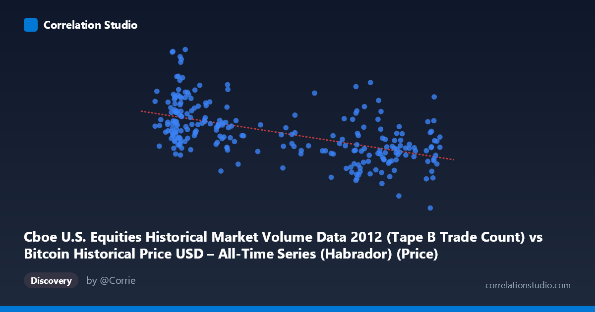
Cboe U.S. Equities Historical Market Volume Data 2012 (Tape B Trade Count) vs Bitcoin Historical Price USD – All-Time Series (Habrador) (Price)
- Pearson correlation (r)
- -0.5602
- Spearman correlation
- -0.5644
- p-value
- 0
- Sample size (n)
- 250
- 95% confidence interval
- -0.6398 to -0.4687
- Granger causality
- None
- Granger optimal lag
- 10
AI analysis
Analysis of Variable Relationship
1. Overview of the Visualization
The scatterplot depicts a moderate negative relationship between the X variable (Tape B Trade Count) and Y variable (Bitcoin Price). As X increases from roughly 4.3 to 13.7, Y tends to decline from highs near $298,000 to lows near $63,000. The data points cluster into two loosely defined regions: a lower-X cluster (values 4.3–7.0) associated with higher Y values (typically 160,000–245,000), and a higher-X cluster (values 9.8–12.6) associated with lower Y values (typically 100,000–175,000). This bimodal clustering, rather than a smooth continuous scatter, suggests the relationship may be driven more by distinct regimes or time periods than by a fine-grained linear mechanism.
2. Strength, Direction, and Statistical Confidence
The correlation coefficient (r = -0.560) indicates a moderate negative linear relationship, with the regression line (y = -6939.76x + 233,168) confirming that Y decreases as X increases. However, r² = 0.314 reveals that only about 31% of the variance in Y is explained by X — meaning nearly 70% of the variability in price is driven by other factors entirely unaccounted for in this bivariate relationship. The 95% confidence interval [-0.640, -0.469] is reasonably tight and excludes zero, and the p-value of ~0 confirms this correlation is statistically significant and not due to random chance in this sample. That said, statistical significance with modest r² means the relationship is real but weak-to-moderate in practical predictive power. Critically, the Granger causality tests show no significant predictive direction in either direction (X→Y: p=0.607; Y→X: p=0.354), meaning that despite the correlation, neither variable helps forecast future values of the other over time. This strongly suggests the correlation is contemporaneous/coincidental rather than causal or dynamically predictive.
3. Notable Patterns and Outliers
The data shows some notable dispersion within clusters — for example, at X≈4.86, Y ranges dramatically from ~172,718 to ~295,122, indicating high variance even at fixed X values. Similarly, at X≈10.92–10.95, Y values swing between ~104,220 and ~207,237. This heteroskedasticity (uneven spread) undermines the strength of a pure linear fit. A few points stand out as potential outliers: (4.86, 295,121.87) is unusually high for its X value, and (11.67, 222,649.67) is unusually high within the high-X cluster where most values are below 175,000. No strong evidence of nonlinear curvature (e.g., quadratic or exponential shape) is apparent — the decline looks roughly linear but noisy.
4. Confounding Factors and Caveats
This pairing is conceptually unusual: it compares U.S. equities market trade counts (Tape B) against Bitcoin's all-time price history, restricted to a 2012 time window. Since Bitcoin was in a very early, low-liquidity, low-price phase in 2012 (pre-major bull runs), any correlation with unrelated equities trade volume is likely spurious, driven by shared time trends rather than any economic linkage. Both series may simply trend over the year (e.g., equities trade counts rising/falling seasonally while Bitcoin price drifted in its own early trajectory), producing a "correlation by coincidence" pattern common in time-series data with autocorrelation. The lack of Granger causality in either direction reinforces this — there's no evidence of a lead-lag mechanism connecting these markets in 2012.
5. Actionable Insights and Further Investigation
Given the weak explanatory power (r²=0.31), lack of Granger causality, and the conceptual mismatch between the datasets (equities trade counts vs. early Bitcoin price), this correlation should not be used for predictive or trading purposes. Analysts should treat this as likely spurious and investigate whether both series are simply non-stationary/trending over 2012 (a common cause of false correlations). Recommended next steps: (a) detrend or difference both series and re-test correlation on stationary data, (b) check for shared macro drivers (e.g., overall market sentiment, USD strength) rather than assuming direct linkage, and (c) if genuine interest exists in equities-crypto relationships, use contemporaneous, overlapping, and liquid periods (post-2017) rather than 2012, when Bitcoin markets were nascent and thinly traded.
X dataset: Bitcoin Historical Price USD – All-Time Series (Habrador)
Y dataset: Cboe U.S. Equities Historical Market Volume Data 2012
Part of experiment: Bitcoin - Bitcoin Historical Price USD – All-Time Series (Habrador) vs Cboe U.S. Equities Historical Market Volume Data 2012