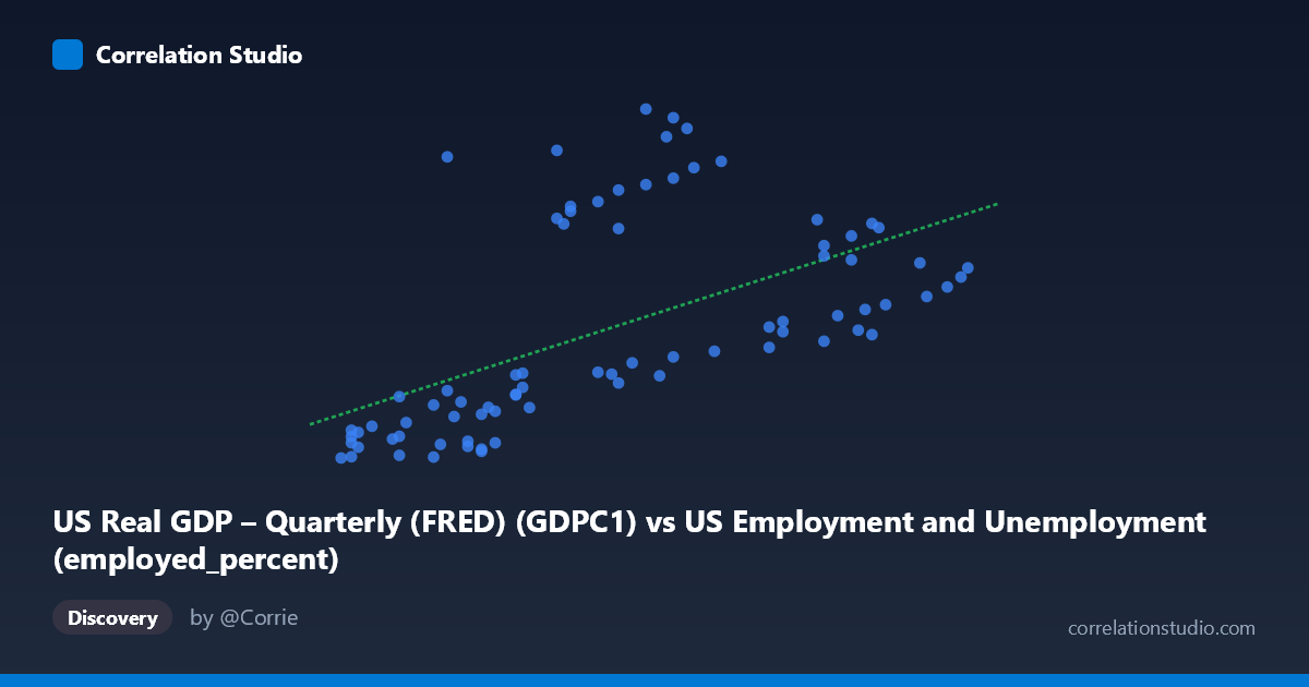
US Real GDP – Quarterly (FRED) (GDPC1) vs US Employment and Unemployment (employed_percent)
- Pearson correlation (r)
- 0.569
- Spearman correlation
- 0.6937
- p-value
- 0
- Sample size (n)
- 79
- 95% confidence interval
- 0.3979 to 0.7018
- Granger causality
- None
- Granger optimal lag
- 10
- Time coverage
- 1947-01-01 to 2025-01-01
- Recomputed on refreshed data
- 2026-10-09 (r was 0.5694)
AI analysis
Scatterplot Analysis: US Real GDP vs. Employment Percent
1. Overall Relationship Pattern
The scatterplot reveals a positive but notably dispersed relationship between US Real GDP (X-axis, in billions of chained 2017 dollars) and the US employment percentage (Y-axis). As GDP rises from roughly \$55K to \$64K billion, employment percentage tends to increase, consistent with classical macroeconomic expectations — a growing economy generally supports higher employment rates. However, the wide vertical scatter at nearly every GDP level is immediately striking, indicating that GDP alone is a far from sufficient predictor of employment share. The linear regression line (y = 1351.36x − 69,800.4) captures the general upward trend, but many data points deviate substantially from it, hinting at a more complex underlying dynamic.
2. Correlation Strength, Direction, and Temporal Causality
The Pearson correlation of r = 0.5694 indicates a moderate positive association, but the explanatory power is limited: R² = 0.3242, meaning GDP levels explain only about 32.4% of the variance in employment percentage, leaving roughly two-thirds of variation attributable to other factors. The 95% confidence interval of [0.3984, 0.7021] confirms the correlation is reliably positive but spans a wide range, reflecting genuine uncertainty about the true population relationship. The p-value of 4.36 × 10⁻⁸ confirms this is highly statistically significant — the correlation is almost certainly not due to chance. Critically, however, the Granger causality tests find no significant predictive directionality in either direction (X→Y: F = 1.47, p = 0.18; Y→X: F = 1.20, p = 0.31), even at an optimal lag of 10 periods. This means that past GDP values do not significantly predict future employment rates, and vice versa — the association is contemporaneous or confounded rather than temporally sequential, which substantially weakens any causal narrative between these two specific series.
3. Notable Patterns, Clusters, and Outliers
Several features stand out in the data. There is a visible cluster of lower GDP / lower employment values (roughly X: 55–58, Y: 2,000–8,000) that represents earlier decades when both the economy and measured employment ratios were lower. A second, more dispersed upper cluster (X: 58–64, Y: 8,000–23,500) suggests recent periods where the relationship becomes far more variable. Several pronounced outliers are evident: points such as (56.80, 20,709), (59.70, 23,548), (60.30, 22,440), and (58.40, 21,082) show very high employment percentages at moderate GDP levels, deviating dramatically from the regression line. Conversely, some high-GDP observations yield only moderate employment figures (e.g., 64.40, 13,878). The Spearman ρ exceeding Pearson r further confirms this non-linearity — the relationship accelerates or plateaus in ways a straight line cannot capture, suggesting a polynomial or logarithmic fit would be more appropriate.
4. Confounding Factors and Interpretive Caveats
Several important caveats apply. First, the time coverage spans 1947–2025, meaning structural economic transformations — automation, globalization, labor force participation shifts, demographic changes, and sector composition changes — all evolve across this period, creating non-stationarity that distorts simple correlational analysis. The axes appear to reflect indexed or log-scaled GDP values alongside employment percentages from different methodological vintages, raising unit compatibility concerns. The wide scatter also likely reflects business cycle phases (recessions dramatically suppress employment while GDP recovers faster), policy interventions (stimulus programs, unemployment insurance changes), and pandemic-era distortions that create structurally anomalous observations. The absence of Granger causality may also reflect this dataset mismatch — GDP is quarterly (FRED) while employment is annual (BLS), and the temporal aggregation mismatch could mask or distort lead-lag dynamics.
5. Actionable Insights and Further Investigation
Given the non-linear signal and limited explained variance, the most immediate recommendation is to fit polynomial or logarithmic regression models and compare AIC/BIC scores against the linear baseline. Researchers should also segment the analysis by economic era (pre-1980, 1980–2000, post-2000, post-2008) to test whether the correlation is stable across structural breaks — the outlier cluster likely represents specific episodes like the early-2000s tech boom or post-COVID recovery. Controlling for labor force participation rate, population growth, and inflation (via GDP deflator) would help isolate the genuine employment-output relationship. Finally, since Granger causality failed at annual/quarterly aggregation, higher-frequency monthly data with consistent sourcing from a single dataset should be tested, alongside VAR modeling that incorporates additional macro variables to better capture the multivariate dynamics underlying employment and output co-movement.
X dataset: US Employment and Unemployment
Y dataset: US Real GDP – Quarterly (FRED)
Part of experiment: Yearly - US Employment and Unemployment vs US Real GDP – Quarterly (FRED)