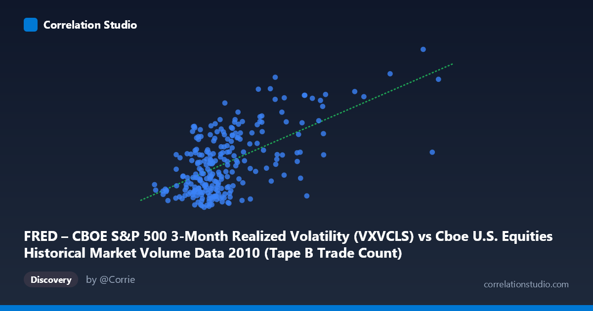
FRED – CBOE S&P 500 3-Month Realized Volatility (VXVCLS) vs Cboe U.S. Equities Historical Market Volume Data 2010 (Tape B Trade Count)
- Pearson correlation (r)
- 0.6059
- Spearman correlation
- 0.4914
- p-value
- 0
- Sample size (n)
- 252
- 95% confidence interval
- 0.5213 to 0.6786
- Granger causality
- Y → X
- Granger optimal lag
- 1
AI analysis
Analysis: CBOE S&P 500 3-Month Realized Volatility vs. Tape B Trade Count (2010)
Relationship Overview The scatterplot reveals a moderate positive relationship between CBOE S&P 500 3-Month Realized Volatility (VXVCLS) and Tape B Trade Count in U.S. equity markets during 2010. As volatility increases, trade counts tend to rise, which aligns with intuitive market dynamics — heightened uncertainty typically drives increased trading activity across exchanges. The linear regression equation (y = 2.12236E-05x + 18.4186) confirms this upward trend, though the scatter around the regression line is substantial, indicating that volatility alone is far from a complete explanation of trading volume behavior.
Correlation Strength and Statistical Significance The Pearson correlation of r = 0.6059 indicates a moderate-to-strong positive association, but the explanatory power is more sobering: r² = 0.3671 means that only ~36.7% of the variance in Tape B Trade Count is explained by realized volatility, leaving nearly two-thirds attributable to other factors. The 95% confidence interval for r of [0.5213, 0.6786] is reasonably tight given n = 252 paired samples from a population of N = 3,302, and the p-value of effectively 0 confirms this relationship is highly unlikely to be a statistical artifact. Critically, the Granger causality results suggest a unidirectional temporal relationship where Y (Tape B Trade Count) Granger-causes X (VXVCLS) — the F-statistic for Y→X is 6.88 (p = 0.0092) versus a non-significant X→Y (F = 3.31, p = 0.0702). This is a notable and somewhat counterintuitive finding: rather than volatility driving trading activity, lagged trade counts appear to predict forward realized volatility more strongly, suggesting that elevated trading volume may be a leading indicator of subsequent volatility regimes.
Patterns, Clusters, and Outliers The scatterplot exhibits a few noteworthy structural features. There appears to be a dense cluster of points at lower X values (roughly 95,000–350,000 range) with Y values concentrated between 18–28, suggesting that during calmer, lower-volume periods, volatility stays rangebound. Beyond approximately 400,000 in trade count, the distribution fans outward, with several high-X, high-Y observations — most notably the point near (918,659, 36.62), which stands as a clear outlier at the extreme right. Additional elevated volatility readings (e.g., 36.91, 37.40, 40.83) paired with high trade counts represent potential stress periods during 2010, possibly associated with the May Flash Crash or European sovereign debt concerns. The spread widens considerably at higher trade counts, hinting at heteroscedasticity — variance in volatility is not constant across the range of trading activity.
Confounding Factors and Caveats Several important caveats complicate direct causal interpretation. First, both variables may be jointly driven by macroeconomic shocks — major news events, earnings seasons, or systemic stress episodes would simultaneously spike both volatility and trading volume, creating spurious correlation. Second, the axis labeling warrants careful attention: the dataset descriptions appear swapped in the metadata (X-axis references VXVCLS but is labeled from the Cboe volume dataset, and vice versa), which could affect interpretive conclusions and should be verified. Third, Tape B specifically covers NYSE American (AMEX) and regional exchange stocks, making it a subset of total market activity — generalization to broader market dynamics should be made cautiously. Finally, the 2010 time window includes the Flash Crash (May 6), a structurally unique event that may disproportionately influence both the correlation and Granger test results.
Actionable Insights and Further Investigation The Granger causality finding — that trade count predicts future volatility rather than the reverse — is the most actionable result here and merits deeper investigation. Practitioners could explore whether elevated Tape B trade counts serve as a practical early-warning signal for volatility spikes, which would have direct relevance for options pricing, risk management, and hedging strategies. Recommended next steps include: (1) extending the analysis beyond 2010 to test whether this Granger relationship is stable across different market regimes; (2) decomposing the heteroscedastic region (high trade counts) to identify whether outlier periods correspond to identifiable market events; (3) testing non-linear models (e.g., log transforms or regime-switching frameworks) given the apparent fan-shaped dispersion; and (4) incorporating additional controls such as VIX levels, macroeconomic announcements, or cross-exchange volume data to better isolate the independent contribution of Tape B activity to volatility forecasting.
X dataset: Cboe U.S. Equities Historical Market Volume Data 2010
Y dataset: FRED – CBOE S&P 500 3-Month Realized Volatility
Part of experiment: Daily - Cboe U.S. Equities Historical Market Volume Data 2010 vs FRED – CBOE S&P 500 3-Month Realized Volatility