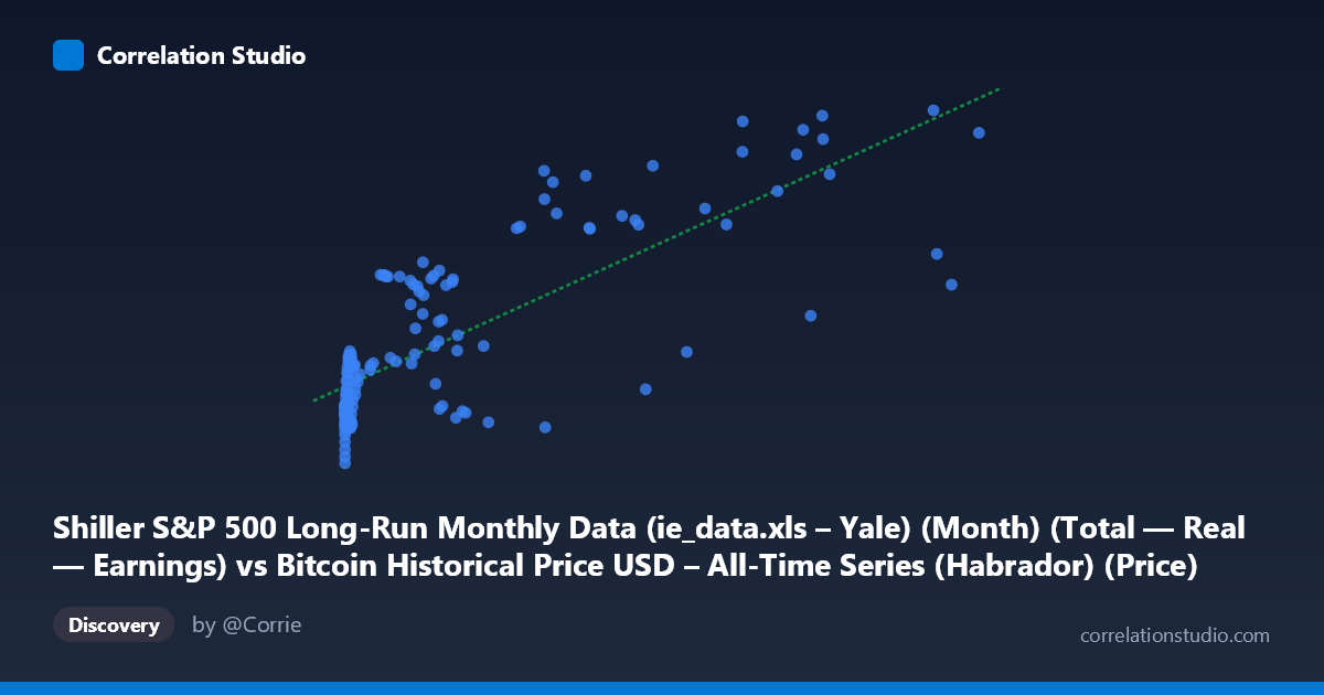
Shiller S&P 500 Long-Run Monthly Data (ie_data.xls – Yale) (Month) (Total — Real — Earnings) vs Bitcoin Historical Price USD – All-Time Series (Habrador) (Price)
- Pearson correlation (r)
- 0.7862
- Spearman correlation
- 0.7709
- p-value
- 0
- Sample size (n)
- 155
- 95% confidence interval
- 0.7174 to 0.8397
- Granger causality
- None
- Granger optimal lag
- 2
- Time coverage
- 2010-08-01 to 2023-06-01
- Recomputed on refreshed data
- 2026-10-24 (r was 0.7862)
AI analysis
Analysis: Bitcoin Price vs. S&P 500 Real Earnings
1. What the Visualization Reveals
The scatterplot shows a positive, non-linear relationship between two variables that are, on their face, economically unrelated: Bitcoin's USD price and Shiller's real S&P 500 earnings data. The data shows a curve rather than a straight line — Y values cluster tightly around 100-140 for small X values (near zero), then rise more steeply as X increases into the tens of thousands. This pattern is a classic signature of two independent time series that both trended upward over the same historical period rather than a genuine causal or mechanistic relationship. Bitcoin's price is naturally near-zero for early X-axis values and both series have grown substantially since 2010-2023.
2. Strength, Direction, and Uncertainty
The linear correlation (r = 0.786, r² = 0.618) indicates that a linear model explains about 62% of the variance in Y, leaving nearly 40% unexplained — a moderate-to-strong but far from complete relationship. The 95% CI [0.717, 0.840] is reasonably tight given n=155, and the p-value of ~0 confirms this correlation is statistically robust and not due to chance. However, statistical significance here should not be conflated with practical meaning: with 1,834 possible population points and highly autocorrelated time series data, artificially narrow confidence intervals and inflated significance are common. Critically, Granger causality tests show no significant predictive direction in either direction (X→Y: p=0.243; Y→X: p=0.538). This is the most important finding: neither series helps forecast the other's future values once past values of both are accounted for. This strongly suggests the correlation is driven by a shared time trend (mutual drift) rather than any lead-lag causal mechanism.
3. Notable Patterns and Outliers
The data shows a clear inflection/threshold pattern: for X < 1,000 (early Yale earnings values), Y (Bitcoin price) stays low and compressed (100-140), consistent with Bitcoin's pre-2017 price history. Beyond X ≈ 10,000, Y increases substantially and with more scatter/volatility (e.g., points like (45092.81, 148.17) vs. (46208.21, 215.46) show huge Y swings for similar X — a sign of heteroscedasticity). Point (45092.81, 148.17) is a notable outlier, breaking from the otherwise upward trend, likely capturing a Bitcoin bear-market month. The relationship also seems to plateau or show diminishing returns at the highest X values (see 61374.28 → 209.69, lower than 46208.21 → 215.46), hinting the true relationship may be logarithmic or saturating rather than linear.
4. Confounding Factors and Caveats
The core caveat: this is very likely a spurious correlation driven by co-trending time series, not a genuine economic relationship. Both Bitcoin price and Shiller earnings data have risen over 2010-2023 due to completely different macro drivers (crypto adoption/speculation vs. corporate earnings growth/inflation). Time itself is an obvious lurking confounder — both series may correlate with calendar time, monetary policy (QE, low rates), inflation, or general market sentiment rather than with each other directly. Additionally, financial time series exhibit strong autocorrelation, which violates the independence assumptions underlying standard p-value/CI calculations, likely overstating the reliability of the reported statistics.
5. Actionable Insights
Rather than treating this as evidence of a meaningful link, analysts should: (1) detrend both series (e.g., using year-over-year returns instead of levels) and recheck correlation — this is the standard test for distinguishing genuine co-movement from shared drift; (2) treat the Granger causality result as decisive — with no predictive direction found, this pairing should not be used for forecasting one from the other; (3) investigate common macro covariates (interest rates, inflation, USD index) that may simultaneously drive both series; and (4) if visualization purposes are the goal, the current framing is fine, but any inference of "Bitcoin tracks stock earnings" or vice versa should be avoided without stronger causal/economic justification.
X dataset: Bitcoin Historical Price USD – All-Time Series (Habrador)
Y dataset: Shiller S&P 500 Long-Run Monthly Data (ie_data.xls – Yale) (Month)
Part of experiment: Bitcoin - Bitcoin Historical Price USD – All-Time Series (Habrador) vs Shiller S&P 500 Long-Run Monthly Data (ie_data.xls – Yale) (Month)