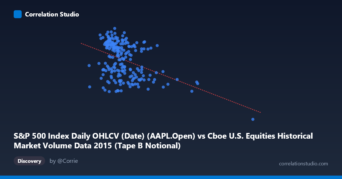
S&P 500 Index Daily OHLCV (Date) (AAPL.Open) vs Cboe U.S. Equities Historical Market Volume Data 2015 (Tape B Notional)
- Pearson correlation (r)
- -0.4129
- Spearman correlation
- -0.3609
- p-value
- 0
- Sample size (n)
- 222
- 95% confidence interval
- -0.5165 to -0.2974
- Granger causality
- None
- Granger optimal lag
- 1
AI analysis
Scatterplot Analysis: AAPL Opening Price vs. Cboe Tape B Notional Volume
Relationship Overview
The scatterplot reveals a moderate negative relationship between Apple's (AAPL) daily opening price on the S&P 500 and Cboe's Tape B notional trading volume for U.S. equities in 2015. The linear regression equation (y = -1.74×10⁻⁹x + 130.335) indicates that as AAPL's opening price increases, Tape B notional volume tends to decrease, and vice versa. This inverse relationship is visually apparent in the scatter, though with considerable dispersion around the trend line. The bulk of observations cluster in the lower X range (roughly $3–7 billion in AAPL open price units), with a long right tail of higher-value outliers pulling the regression line.
Correlation Strength and Statistical Significance
The Pearson correlation of r = -0.4129 reflects a moderate negative association, but the explanatory power is modest: r² = 0.1705, meaning only 17.1% of the variance in Tape B notional volume is explained by AAPL's opening price. The remaining ~83% of variation is attributable to other factors entirely. The 95% confidence interval of [-0.5165, -0.2974] is entirely negative, confirming the direction of the relationship, and the extremely small p-value (1.5×10⁻¹⁰) indicates this correlation is highly unlikely to be a chance finding given n = 222 paired observations. Despite statistical significance, practical significance is limited. Critically, Granger causality tests show no significant directional predictive relationship in either direction (X→Y: F = 0.795, p = 0.374; Y→X: F = 1.156, p = 0.284), meaning neither variable reliably predicts the other temporally at a one-period lag. The correlation should therefore not be interpreted as evidence that one drives the other in any causal or forecasting sense.
Notable Patterns, Clusters, and Outliers
Several features stand out visually. The majority of data points form a dense cluster in the X range of approximately 3.5–7.0 billion, with Y values spanning roughly 107–134, exhibiting wide vertical scatter that reinforces the weak-to-moderate fit. There are at least two prominent outliers at extreme X values: one point near X ≈ 17.9 billion with a notably low Y value (~94.87), and another near X ≈ 12.5 billion with Y ≈ 111. These high-leverage points likely exert disproportionate influence on the regression slope and the overall correlation coefficient. There also appears to be a potential non-linear feature — the relationship may steepen at higher X values — suggesting a simple linear model may not fully capture the dynamics across the full range. A small cluster of high-Y values (Y 130) appears concentrated at moderate X values (~3.9–5.4 billion), possibly reflecting specific market events during the February–December 2015 coverage window.
Confounding Factors and Caveats
Several important caveats apply. First, the axis labels appear inverted relative to dataset descriptions — the X-axis draws from the Cboe market volume dataset while the Y-axis draws from the S&P 500 OHLCV dataset — which warrants verification before drawing conclusions. Second, both variables are time-series data over 2015, meaning common temporal trends (e.g., market volatility events like the August 2015 correction) could simultaneously affect both, creating spurious correlation driven by shared macroeconomic shocks rather than any direct relationship. Third, AAPL opening price is a single-stock metric being compared to a broad market tape metric; index composition effects, sector rotations, and liquidity conditions could all act as confounders. Finally, the sample covers only n = 222 of N = 506 total observations, and the sampling method (every 4th point) may introduce systematic gaps that affect representativeness.
Actionable Insights and Further Investigation
Given the lack of Granger causality, this correlation should not be used for predictive trading strategies in either direction without substantially more evidence. Investigators should consider: (1) removing or separately modeling the high-leverage outliers (particularly the ~17.9B observation) to assess whether the correlation holds robustly; (2) testing non-linear models (logarithmic or polynomial) that may better capture curvature at high X values; (3) incorporating additional market microstructure variables — VIX levels, overall market volume, or sector-specific flows — as control variables to isolate whether any meaningful partial correlation survives; and (4) conducting rolling-window correlation analysis across the 2015 timeline to determine whether the relationship strengthens during high-volatility periods (e.g., August 2015), which would suggest event-driven co-movement rather than a structural link.
X dataset: Cboe U.S. Equities Historical Market Volume Data 2015
Y dataset: S&P 500 Index Daily OHLCV (Date)
Part of experiment: Daily - Cboe U.S. Equities Historical Market Volume Data 2015 vs S&P 500 Index Daily OHLCV (Date)