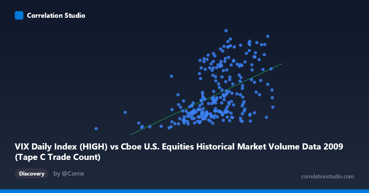
VIX Daily Index (HIGH) vs Cboe U.S. Equities Historical Market Volume Data 2009 (Tape C Trade Count)
- Pearson correlation (r)
- 0.4991
- Spearman correlation
- 0.535
- p-value
- 0
- Sample size (n)
- 252
- 95% confidence interval
- 0.4002 to 0.5865
- Granger causality
- None
- Granger optimal lag
- 1
- Time coverage
- 2009-01-02 to 2009-12-31
- Recomputed on refreshed data
- 2026-10-09 (r was 0.4991)
AI analysis
Scatterplot Analysis: VIX Daily Index (HIGH) vs. Tape C Trade Count (2009)
Overview of the Relationship
The scatterplot reveals a moderate positive relationship between the VIX Daily Index High values and the Tape C Trade Count across U.S. equity exchanges during 2009. As VIX High values increase, Tape C trade counts tend to rise as well, consistent with the well-established market microstructure intuition that elevated volatility environments drive higher trading activity. The linear regression equation (y = 4.80×10⁻⁵x + 2.26) reflects this upward slope, though the considerable scatter around the regression line immediately signals that the relationship is far from deterministic. The data spans the full calendar year 2009, a period that encompassed both the tail end of the Global Financial Crisis and the subsequent market recovery — a context that is crucial for interpreting any patterns observed.
Correlation Strength, Direction, and Statistical Framing
The Pearson correlation of r = 0.4991 indicates a moderate positive association, but the more practically meaningful figure is r² = 0.2491, meaning that VIX High values explain only about 25% of the variance in Tape C trade counts. The remaining 75% of variability is attributable to factors entirely outside this bivariate relationship. The 95% confidence interval for r of [0.40, 0.59] is reasonably tight given the sample size of n = 252, suggesting the true population correlation is unlikely to be trivially small or implausibly large, and the p-value of effectively zero confirms this is not a chance finding in a statistical sense. However, the Granger causality results introduce an important caveat: neither direction of temporal prediction (X→Y or Y→X) achieves significance at even conventional thresholds (F = 0.41, p = 0.52 for X→Y; F = 0.01, p = 0.91 for Y→X at lag 1). This means that past VIX High values do not reliably predict future trade counts, and vice versa — the contemporaneous correlation exists, but there is no exploitable lead-lag predictive relationship between the two series at a one-period lag.
Notable Patterns, Clusters, and Outliers
Several structural features stand out in the scatterplot. There is a visible cluster of observations at lower VIX values (roughly 185,000–600,000 range on the X-axis) paired with relatively low trade counts (approximately 20–32), reflecting the calmer, recovering market conditions in the second half of 2009. A second, more dispersed cluster appears at higher VIX values with elevated trade counts, consistent with the crisis-period volatility spikes in early 2009. Notably, a few outliers warrant attention: the point near (185,886, 19.67) sits far to the left and represents an unusually low VIX reading paired with a minimal trade count, while several points in the upper-right quadrant (e.g., around (806,023, 51.95) and (761,867, 53.25)) show both extremely high VIX readings and very high trade counts. Interestingly, the relationship also shows heteroscedasticity — the spread of trade count values appears to fan outward at higher VIX levels, suggesting the variance of trading activity is itself a function of volatility regime.
Confounding Factors and Interpretive Caveats
Several important confounds complicate a causal reading of this correlation. 2009 was a structurally atypical year: the first quarter captured peak crisis stress, while the latter quarters reflected a sharp recovery rally, meaning the year-level data conflates two fundamentally different market regimes. This regime shift alone could artificially inflate the correlation by creating two distinct clusters that a single regression line connects. Additionally, Tape C specifically covers NASDAQ-listed securities, which may behave differently from the broader market. Macroeconomic news releases, Federal Reserve interventions, earnings cycles, and month-end rebalancing flows all independently influence both VIX levels and trading volumes, acting as common drivers rather than causal mechanisms linking these two variables directly. The fact that the VIX dataset labels and axis assignments appear inverted (VIX data described under the trade count axis and vice versa) also warrants verification to ensure the variables are mapped correctly before drawing firm conclusions.
Actionable Insights and Further Investigation
Given these findings, several investigative paths are worth pursuing. Regime-segmented analysis — splitting the data into crisis (Q1 2009) and recovery (Q2–Q4 2009) sub-periods — would clarify whether the correlation is driven primarily by one regime or holds consistently across both. Extending the Granger causality testing to multiple lags (beyond lag 1) could reveal delayed predictive relationships that the single-lag test misses. Researchers should also consider controlling for contemporaneous confounders such as S&P 500 returns, macro data release days, and Federal Reserve announcement dates using a multivariate regression framework. Finally, comparing Tape C with Tape A and Tape B trade counts would test whether the relationship is idiosyncratic to NASDAQ-listed securities or a broader market phenomenon, providing more robust and actionable intelligence for trading operations or risk management decisions.
X dataset: Cboe U.S. Equities Historical Market Volume Data 2009
Y dataset: VIX Daily Index
Part of experiment: Daily - Cboe U.S. Equities Historical Market Volume Data 2009 vs VIX Daily Index