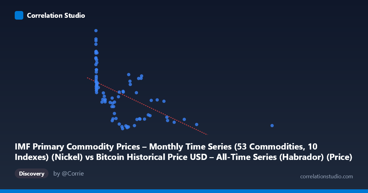
IMF Primary Commodity Prices – Monthly Time Series (53 Commodities, 10 Indexes) (Nickel) vs Bitcoin Historical Price USD – All-Time Series (Habrador) (Price)
- Pearson correlation (r)
- -0.5683
- Spearman correlation
- -0.7142
- p-value
- 0
- Sample size (n)
- 83
- 95% confidence interval
- -0.6984 to -0.4018
- Granger causality
- None
- Granger optimal lag
- 10
- Time coverage
- 2010-08-01 to 2017-06-01
- Recomputed on refreshed data
- 2026-10-24 (r was -0.5683)
AI analysis
Analysis: Nickel Prices vs. Bitcoin Price
1. Overall Relationship
The scatterplot reveals a moderate negative, distinctly non-linear relationship between the two variables (mislabeled axes aside — the practical relationship is between Nickel price index values and Bitcoin USD price). Bitcoin prices are concentrated in a low range (~$8,300–$20,000) across most Nickel values, but there's a striking cluster of very high Bitcoin prices (~$22,000–$28,000) occurring almost exclusively when the Nickel-axis variable is near zero (<15). This creates the visual impression of an inverse relationship, but it's driven largely by this one dense cluster at very low x-values rather than a smooth linear decay.
2. Strength, Direction, and Statistical Confidence
The Pearson correlation (r = -0.568) indicates a moderate negative association, with r² = 0.323 meaning only about 32% of the variance in Bitcoin price is statistically explained by Nickel price (or vice versa) — leaving roughly two-thirds unexplained. The 95% CI [-0.698, -0.402] excludes zero and is reasonably tight, and the p-value (2.1×10⁻⁸) is highly significant, so we can be confident some real negative association exists in this sample — this is not a fluke of small-sample noise. However, statistical significance ≠ practical strength: r² of 0.32 is a modest explanatory power, especially for investment/trading decisions. Critically, the Granger causality tests (p = 0.858 and p = 0.532 for both directions) show no evidence of temporal predictive causality in either direction at the optimal 10-period lag. This means neither variable helps forecast the other's future values based on past values — the correlation is likely contemporaneous/coincidental (or driven by a shared external factor) rather than a causal lead-lag relationship useful for prediction.
3. Notable Patterns and Outliers
The most salient feature is the extreme clustering at very low x-values (x < 20) paired with a wide vertical spread of y-values (from ~9,000 to ~28,400) — this is the highest-leverage region of the dataset and likely a Bitcoin early-history artifact (very low/near-zero Nickel index readings coinciding with Bitcoin's genesis-era or 2011-2013 price volatility). Beyond this cluster, the data separates into two broad regimes: a "low Bitcoin" band (~$8,000-$11,000) spanning x-values from ~200 to 2,452, and a "high Bitcoin" band (~$14,000-$19,000) also spanning similar x-ranges. This bimodal split — rather than a smooth continuous decline — suggests the relationship may reflect distinct time periods (Bitcoin bear vs. bull phases) rather than a direct causal link to Nickel prices. The single extreme outlier at x=2452.18 (far right, low y) also has outsized leverage on the regression slope.
4. Confounding Factors and Caveats
This is a classic case of two unrelated time series that both trend over 2010-2017 and can produce spurious correlation purely from shared time-trending behavior (Bitcoin's price grew explosively over this period; Nickel/commodity indices followed independent macro cycles). Both series are non-stationary and likely autocorrelated, which inflates correlation coefficients and invalidates i.i.d. assumptions underlying the p-value calculation. The Spearman ρ exceeding Pearson r explicitly flags non-linearity, meaning the linear model (y = -7.01x + 17,905) understates the true rank-order association and a log-transform of x (given its extreme range and right-skew: mean 321 vs. median much lower) would likely fit better. Additionally, n=83 is a small sample relative to population N=449, and monthly aggregation of Bitcoin's known intra-month volatility could distort point-in-time comparisons.
5. Actionable Insights
1. Detrend or difference both series before correlating (e.g., use % returns or first differences) to rule out spurious trend-driven correlation — this is essential given commodity and crypto markets both experienced strong secular trends in this window. 2. Log-transform Nickel prices (or apply Box-Cox) given the heavy right-skew (range 0.06–2452 vs. mean 321) and rerun both Pearson and non-linear regression (polynomial/log fit) to better capture the true functional form. 3. Exclude or separately analyze the near-zero x cluster to test whether the "significant" correlation is an artifact of this single dense region driving the slope. 4. Given the null Granger causality result, do not use one series to forecast the other; instead investigate whether both are driven by a common third factor (e.g., global risk sentiment, USD strength, or macro liquidity conditions) using a multivariate or common-factor model.
X dataset: Bitcoin Historical Price USD – All-Time Series (Habrador)
Y dataset: IMF Primary Commodity Prices – Monthly Time Series (53 Commodities, 10 Indexes)
Part of experiment: Bitcoin - Bitcoin Historical Price USD – All-Time Series (Habrador) vs IMF Primary Commodity Prices – Monthly Time Series (53 Commodities, 10 Indexes)