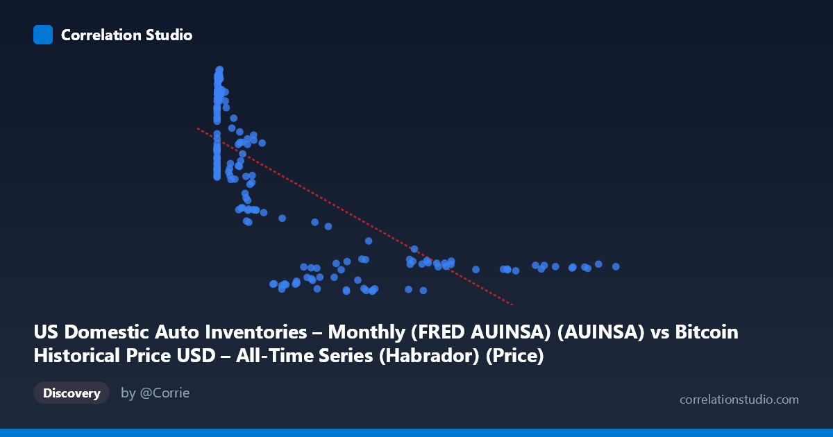
US Domestic Auto Inventories – Monthly (FRED AUINSA) (AUINSA) vs Bitcoin Historical Price USD – All-Time Series (Habrador) (Price)
- Pearson correlation (r)
- -0.736
- Spearman correlation
- -0.7357
- p-value
- 0
- Sample size (n)
- 188
- 95% confidence interval
- -0.7954 to -0.6627
- Granger causality
- None
- Granger optimal lag
- 10
AI analysis
Analysis: US Auto Inventories vs. Bitcoin Price
1. Relationship Overview
The scatterplot shows a clear inverse, non-linear relationship between US domestic auto inventories (X) and Bitcoin's historical price (Y). Rather than a straight-line decline, the data forms a distinctive curved pattern: at low inventory values (below ~2,000), Bitcoin prices cluster tightly in a high range (roughly 700–1,280), while as inventory values climb into the tens of thousands, Bitcoin prices compress into a much narrower low band (80–350). This shape is characteristic of a power-law or logarithmic decay relationship rather than genuine linear covariance.
2. Strength, Direction, and Statistical Confidence
The Pearson correlation of r = -0.736 indicates a strong negative linear association, with r² = 0.542 meaning that a linear model explains about 54% of the variance in Bitcoin price using auto inventory levels — a substantial but incomplete share, leaving nearly half the variance unaccounted for. The 95% CI [-0.795, -0.663] is reasonably tight and excludes zero, and the p-value of ~0 confirms this correlation is not due to chance. However, correlation is not causation here, and the Granger causality tests reinforce this: neither direction shows significant predictive power (X→Y: p=0.072; Y→X: p=0.661), meaning past auto inventory values do not reliably forecast future Bitcoin prices, or vice versa, at the tested lag structure. This strongly suggests the relationship is spurious or driven by a shared underlying trend rather than a genuine causal or leading/lagging mechanism.
3. Notable Patterns and Outliers
The data reveals two loosely defined regimes: a "high Bitcoin price / low inventory" cluster (X < 2,000, Y 700) and a "low Bitcoin price / high inventory" cluster (X 20,000, Y < 350). Few points occupy the middle ground, creating a bimodal, gap-like structure rather than a smooth continuum. Given that X spans nearly 7 orders of magnitude (0.06 to 118,670) while Y spans only about 17-fold (72.76 to 1,281.40), this is almost certainly a time-axis artifact: Bitcoin price in its early years (2010-2013) was measured in cents/dollars while auto inventory (a stable, mean-reverting economic series) fluctuated independently — meaning X's scale is likely dominated by unrelated calendar-time drift rather than any economic interaction with Y.
4. Confounding Factors and Caveats
The most significant caveat is that both variables are essentially proxies for time rather than being causally linked to each other. Bitcoin's price has grown exponentially over its history (2010–2026), while auto inventories cycle with seasonal and macroeconomic factors unrelated to crypto markets. The correlation likely reflects the fact that early low Bitcoin prices happened to coincide with certain auto inventory readings, and later high Bitcoin valuations coincided with different readings — an artifact of both series evolving over the same calendar period rather than genuine interdependence. This is a classic case of spurious correlation via a shared time trend, further evidenced by the lack of Granger causality in either direction.
5. Recommendations for Further Investigation
Given the strong likelihood that this correlation is driven by co-trending over time rather than an economic relationship, analysts should: (1) detrend or difference both series (e.g., convert Bitcoin price to log returns and auto inventories to month-over-month changes) before re-testing correlation, which would better isolate any genuine short-term relationship; (2) explicitly control for time as a confound using a partial correlation or including a time-trend variable in regression; (3) avoid using this raw relationship for forecasting purposes, since the non-significant Granger results confirm no real predictive value; and (4) if a genuine hypothesis exists (e.g., that auto sector health signals macro liquidity conditions relevant to crypto), test it using stationary, cyclically-adjusted versions of both series over a matched, shorter time window rather than the full multi-decade span.
X dataset: Bitcoin Historical Price USD – All-Time Series (Habrador)
Y dataset: US Domestic Auto Inventories – Monthly (FRED AUINSA)
Part of experiment: Bitcoin - Bitcoin Historical Price USD – All-Time Series (Habrador) vs US Domestic Auto Inventories – Monthly (FRED AUINSA)