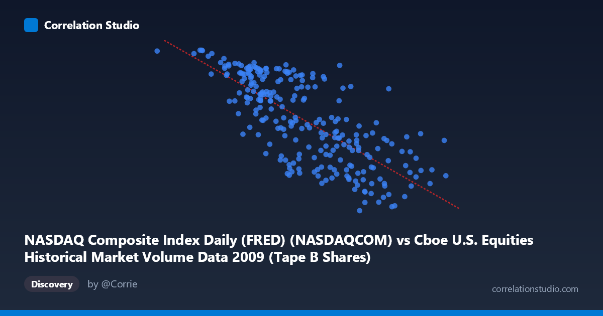
NASDAQ Composite Index Daily (FRED) (NASDAQCOM) vs Cboe U.S. Equities Historical Market Volume Data 2009 (Tape B Shares)
- Pearson correlation (r)
- -0.7481
- Spearman correlation
- -0.7579
- p-value
- 0
- Sample size (n)
- 252
- 95% confidence interval
- -0.7979 to -0.6881
- Granger causality
- Bidirectional
- Granger optimal lag
- 10
AI analysis
Analysis: NASDAQ Composite Index vs. Cboe Tape B Share Volume (2009)
Relationship Overview The scatterplot reveals a clear negative relationship between the NASDAQ Composite Index level and Cboe Tape B share volume during 2009. As the NASDAQ index rose from its crisis lows (around 33.8M on the transformed scale) toward recovery levels (~255.8M), Tape B share volume systematically declined. This pattern is visually consistent with a downward-sloping linear trend, capturing the well-documented phenomenon of panic-driven volume: during market distress early in 2009, trading activity surged, while the subsequent recovery rally was accompanied by declining volume — a classic bear-market-bounce signature.
Correlation Strength and Statistical Significance The Pearson correlation of r = -0.748 is moderate-to-strong and negative, with the linear regression (y = -4.73×10⁻⁶x + 2539.3) explaining R² = 55.96% of the variance in Tape B volume — meaning roughly 44% of volume variability remains unexplained by index level alone. The 95% confidence interval of [-0.798, -0.688] is meaningfully narrow given n = 252, and the p-value of essentially zero confirms this is not a chance finding in the sample. Extrapolating to the broader population (N = 3,232), this relationship appears robust. The bidirectional Granger causality result is particularly noteworthy: at a 10-period lag, both X→Y (F = 2.19, p = 0.019) and Y→X (F = 2.46, p = 0.008) are statistically significant, suggesting the relationship is not simply one-directional. Volume predicting future index levels (Y→X) aligns with market microstructure theory, where volume precedes price moves; index levels predicting future volume (X→Y) reflects sentiment-driven participation cycles.
Notable Patterns and Outliers Several features stand out in the sample points. The lower-left cluster (e.g., x ≈ 33.8M, y = 2285; x ≈ 66.8M, y = 2291) represents early 2009 crisis conditions — extremely low index values paired with very high Tape B volume, consistent with peak-fear selling. Conversely, upper-right points (e.g., x ≈ 243M–255M, y ≈ 1441–1716) reflect late-2009 recovery with compressed volume. There is also notable vertical scatter at mid-range X values (roughly 110M–175M), where Y ranges from ~1442 to ~2194 — a spread of over 750 index points at similar volume levels. This heteroscedasticity suggests the linear model fits less precisely in the mid-range and hints at possible non-linear dynamics or regime shifts during the March 2009 market bottom.
Confounding Factors and Caveats Several important caveats apply. First, 2009 is a highly anomalous year — spanning the tail end of the Global Financial Crisis and a historic recovery — making these dynamics potentially non-generalizable to normal market conditions. Second, Tape B specifically covers NYSE American (AMEX) and regional exchange stocks, which may behave differently from the broader NASDAQ universe the index represents, introducing a cross-dataset definitional mismatch. Third, the bidirectional Granger causality, while statistically significant, uses an optimal lag of 10 periods; this is an empirically chosen lag that may reflect data-fitting rather than a structural economic mechanism. Finally, omitted variables — such as VIX (volatility index), Federal Reserve interventions (QE1 announcement March 2009), or institutional rebalancing flows — likely drive both series simultaneously, inflating the apparent bivariate correlation.
Actionable Insights and Further Investigation Practitioners should resist interpreting this correlation as a stable trading signal without further validation. Recommended next steps include: (1) incorporating VIX or realized volatility as a control variable to partial out fear-driven volume effects; (2) segmenting the analysis into pre- and post-March 2009 bottom regimes to test whether the correlation holds symmetrically in both crisis and recovery phases; (3) extending the Granger analysis across multiple years to assess whether bidirectional predictability persists outside crisis periods; and (4) testing non-linear specifications (e.g., a logarithmic or piecewise regression), given the visible heteroscedasticity at mid-range values. The 44% unexplained variance represents a meaningful opportunity for model enrichment beyond index level alone.
X dataset: Cboe U.S. Equities Historical Market Volume Data 2009
Y dataset: NASDAQ Composite Index Daily (FRED)
Part of experiment: Daily - Cboe U.S. Equities Historical Market Volume Data 2009 vs NASDAQ Composite Index Daily (FRED)