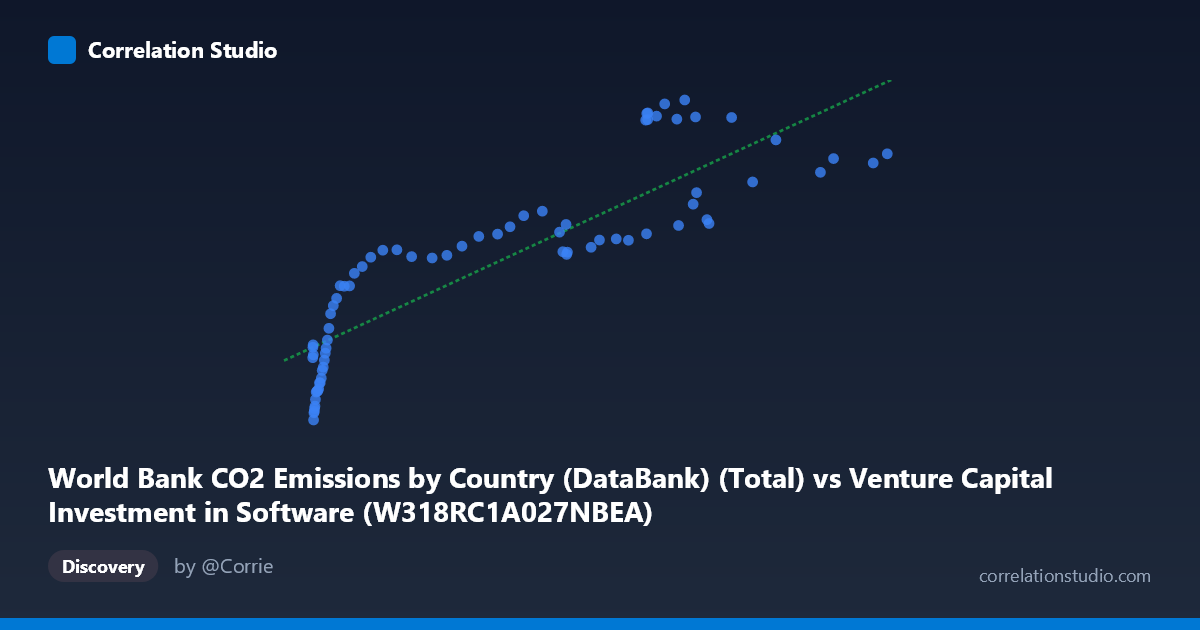
World Bank CO2 Emissions by Country (DataBank) (Total) vs Venture Capital Investment in Software (W318RC1A027NBEA)
- Pearson correlation (r)
- 0.8662
- Spearman correlation
- 0.9273
- p-value
- 0
- Sample size (n)
- 75
- 95% confidence interval
- 0.7957 to 0.9136
- Granger causality
- None
- Granger optimal lag
- 10
- Time coverage
- 1946-01-01 to 2020-01-01
- Recomputed on refreshed data
- 2026-10-24 (r was 0.8662)
AI analysis
Scatterplot Analysis: Venture Capital Software Investment vs. CO₂ Emissions
1. Overall Relationship
The scatterplot reveals a clear positive relationship between the two variables — as CO₂ emissions increase, venture capital investment in software tends to rise as well. The linear regression equation (y = 59.294x + 17,374.1) confirms this upward trajectory, with a relatively steep slope suggesting that each unit increase in CO₂ emissions is associated with a meaningful increase in software investment. However, the relationship is not purely linear; there are visible signs of curvature and clustering that suggest the underlying dynamic is more complex than a simple straight-line model captures. The data spans 1946–2020, meaning this relationship reflects roughly three-quarters of a century of parallel economic and industrial development.
2. Correlation Strength, Direction, and Causality
The Pearson correlation of r = 0.8662 indicates a strong positive association, and the R² of 0.7504 means that approximately 75% of the variance in software VC investment is statistically explained by CO₂ emissions levels — a remarkably high figure for two variables that are not intuitively linked by direct mechanism. The 95% confidence interval for r of [0.7957, 0.9136] is relatively narrow and sits entirely in strongly positive territory, lending high statistical confidence to the association. The p-value of essentially zero confirms this is not a chance finding given the sample size (n = 75). That said, the Granger causality results are unambiguous in their null finding: neither direction of temporal prediction achieves significance (X→Y: F = 0.6744, p = 0.7417; Y→X: F = 0.9486, p = 0.5000). This means that despite the strong contemporaneous correlation, neither variable reliably predicts the other's future values — a critical caveat against any causal narrative, even a directional one.
3. Notable Patterns, Clusters, and Outliers
Several structural features stand out upon closer inspection:
- A dense low-X cluster exists between X ≈ 0.85–50 and Y ≈ 9,870–26,000, corresponding likely to earlier decades (1946–1980s) when both emissions and software investment were comparatively modest. Within this cluster, Y values are quite variable relative to X, suggesting high noise at low emission levels. - A mid-range plateau region around X = 200–300 shows Y values that fan out considerably — some points hover near 27,000–30,000 while others spike to 41,000–43,000 (e.g., the points at approximately (270.67, 41,037), (302.31, 43,129), (286.07, 42,721)). This bimodal vertical spread at similar X values suggests two distinct behavioral regimes in the data, possibly reflecting different eras or structural breaks. - High-X points (X 350) generally cluster between Y = 34,000–39,000, showing a noticeably flatter slope than the mid-range, hinting at a diminishing-returns or saturation effect at the upper end. - The point (302.31, 43,129.15) stands out as a potential high-leverage outlier, with Y well above the regression line's predicted value, which warrants individual inspection.
4. Confounding Factors and Interpretive Caveats
The most important caveat here is that both variables are almost certainly driven by a common third factor: overall economic growth and industrialization over time. As economies expand, they simultaneously burn more fossil fuels and generate more capital for technology investment — making this a textbook example of a spurious correlation mediated by GDP or time trend. The dataset spans 1946–2020, a period of near-monotonic growth in both variables globally, meaning much of the r = 0.866 signal may simply reflect shared temporal trend (non-stationarity) rather than any meaningful structural link. Additionally, the column label mismatch in the metadata — where the X-axis dataset is labeled "Venture Capital Investment in Software" but the column description says CO₂ emissions, and vice versa — introduces the possibility of a data labeling or join error that should be verified before drawing any conclusions. The optimal lag of 10 periods with no significant Granger result also suggests the variables move together contemporaneously due to shared drivers, not sequentially.
5. Actionable Insights and Further Investigation
Given these findings, the following investigative steps are strongly recommended:
- Detrend both series (e.g., first-differencing or HP filter) to remove the shared time trend and retest correlation on the stationary residuals — the true r may be substantially lower than 0.866. - Verify data labeling integrity: the axis-to-dataset description mismatch should be audited immediately to confirm the correct variables are being compared. - Introduce GDP or total energy consumption as a control variable in a multivariate regression to determine whether the CO₂–VC relationship persists after accounting for the most obvious confound. - Investigate the mid-range bifurcation (the cluster of high-Y outliers around X = 270–310) by tagging data points by decade or country — this spread may reflect a structural break such as the dot-com boom of the late 1990s. - Test non-linear models (log-log, square root transformation) given the apparent curvature and heteroscedasticity visible in the scatterplot, which may yield a better fit than the current linear R² of 0.75.
X dataset: Venture Capital Investment in Software
Y dataset: World Bank CO2 Emissions by Country (DataBank)
Part of experiment: Yearly - Venture Capital Investment in Software vs World Bank CO2 Emissions by Country (DataBank)