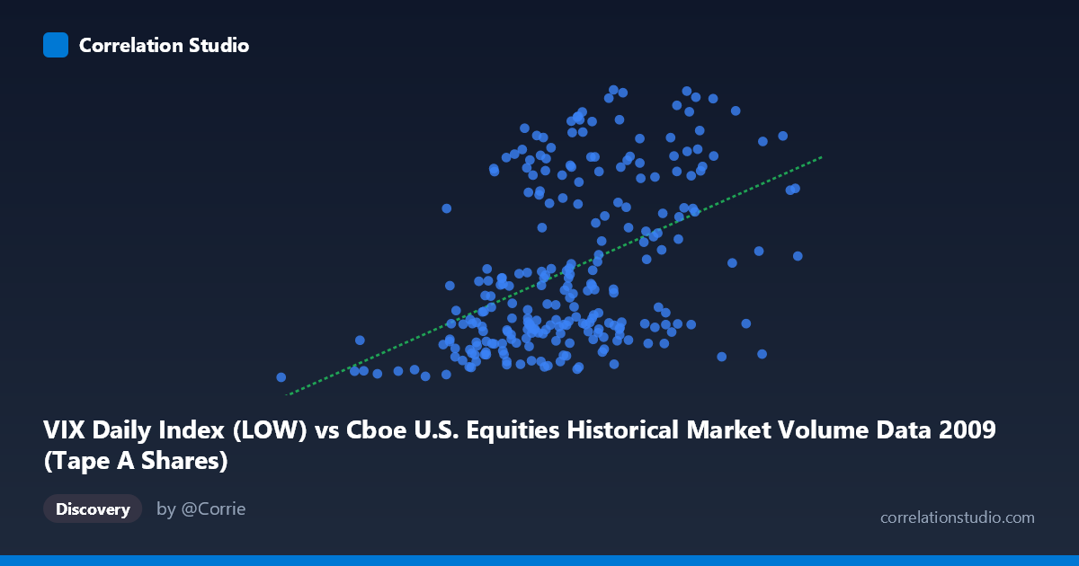
VIX Daily Index (LOW) vs Cboe U.S. Equities Historical Market Volume Data 2009 (Tape A Shares)
- Pearson correlation (r)
- 0.4568
- Spearman correlation
- 0.4717
- p-value
- 0
- Sample size (n)
- 252
- 95% confidence interval
- 0.3531 to 0.5493
- Granger causality
- None
- Granger optimal lag
- 1
- Time coverage
- 2009-01-02 to 2009-12-31
- Recomputed on refreshed data
- 2026-10-09 (r was 0.4568)
AI analysis
Scatterplot Analysis: VIX Tape A Shares vs. VIX Daily Index Low
Relationship Overview
The scatterplot reveals a moderate positive relationship between the VIX Daily Index Low (X-axis, representing daily low volatility readings) and Tape A Share volume from Cboe U.S. Equities Historical Market data (Y-axis). As the VIX low values increase — roughly spanning from ~105M to ~704M in their scaled representation — Tape A share counts tend to drift upward as well. The linear regression equation (y = 4.018×10⁻⁸x + 12.83) confirms this positive slope, though the wide scatter around the regression line immediately signals that the relationship is far from deterministic. This is broadly consistent with the well-established financial intuition that elevated market volatility tends to coincide with increased trading activity, as participants react to uncertainty with heavier buying and selling.
Correlation Strength and Statistical Significance
The Pearson correlation of r = 0.4568 indicates a moderate positive association, but the r² value of 0.2086 is the more telling statistic — it means that only about 20.9% of the variance in Tape A share volume is explained by the VIX low. The remaining ~79% of variance is attributable to other factors entirely, underscoring that while the relationship is real, it is far from a complete explanation. The 95% confidence interval of [0.3531, 0.5493] is meaningfully above zero and relatively tight given the sample size of n = 252 drawn from a population of N = 3,232, suggesting the estimate is stable. The p-value of 2.154×10⁻¹⁴ confirms the correlation is highly statistically significant and almost certainly not a sampling artifact. However, the Granger causality tests complicate the narrative considerably: neither direction (X→Y: F = 0.303, p = 0.583; Y→X: F = 0.942, p = 0.333) reaches significance at conventional thresholds, meaning that neither variable reliably predicts the other's future values at a one-period lag. Statistical correlation and temporal predictive power are telling different stories here.
Visual Patterns, Clusters, and Outliers
The scatterplot exhibits a bimodal vertical banding pattern that is immediately striking. Data points appear to cluster into two distinct horizontal bands: a lower cluster concentrated roughly between Y ≈ 19–30 (lower Tape A share activity) and an upper cluster around Y ≈ 37–49 (higher Tape A share activity), with a relative gap in the mid-30s range. This bifurcation suggests the data may not follow a simple linear relationship and could reflect two distinct market regimes — perhaps pre- and post-crisis stabilization phases within 2009, or systematic differences between high- and low-volatility trading sessions. Several notable outliers are visible at the extremes: the point near X = 105M, Y = 19.25 represents the minimum on both dimensions, while points near X = 606M, Y = 48.35 and X = 501M, Y = 48.97 sit at the high end of the Y distribution. The point at X = 704M, Y = 31.91 is a potential leverage point — the highest X value but with only a middling Y value — which could be moderating the regression slope.
Confounding Factors and Caveats
Several important caveats apply to this analysis. First, the axis labeling appears inverted in the metadata — the X-axis is labeled as "VIX Daily Index Low" from a market volume dataset, while the Y-axis is labeled "Tape A Shares" from a VIX dataset, which likely reflects a data joining artifact rather than a true reversal of variable roles. This ambiguity warrants careful data provenance review before drawing firm conclusions. Second, 2009 was an extraordinary market year, spanning the tail end of the 2008 financial crisis, the March 2009 market trough, and a subsequent strong recovery — meaning the dynamic range of both volatility and volume was unusually compressed in some periods and extreme in others. This temporal heterogeneity may be driving the apparent bimodal clustering. Third, the absence of Granger causality at a one-period lag does not rule out relationships at longer lags, intraday dynamics, or nonlinear causal structures that standard Granger testing would miss.
Actionable Insights and Further Investigation
Given these findings, several investigative steps are warranted. First, testing for a structural break around March 2009 (the market bottom) could determine whether the bimodal clustering reflects two distinct temporal regimes, which would justify fitting separate regression models for each period. Second, nonlinear or polynomial regression should be evaluated, as the visual clustering pattern suggests a simple linear model may be underfitting the true structure. Third, Granger causality should be re-tested at lags of 2–5 periods to rule out slower feedback loops, and multivariate models incorporating additional controls (e.g., S&P 500 returns, trading halts, macroeconomic announcements) could substantially improve explanatory power beyond the current 20.9% R². Finally, verifying the axis-dataset alignment in the source data pipeline should be treated as a priority data quality check before this analysis informs any trading or operational decisions.
X dataset: Cboe U.S. Equities Historical Market Volume Data 2009
Y dataset: VIX Daily Index
Part of experiment: Daily - Cboe U.S. Equities Historical Market Volume Data 2009 vs VIX Daily Index