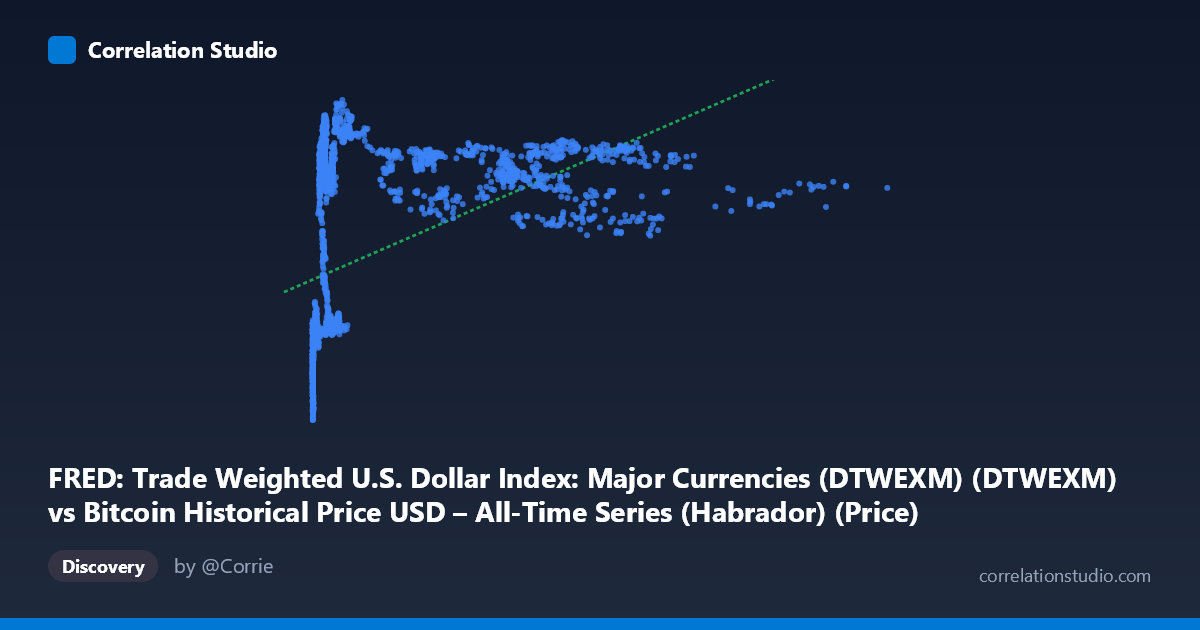
FRED: Trade Weighted U.S. Dollar Index: Major Currencies (DTWEXM) (DTWEXM) vs Bitcoin Historical Price USD – All-Time Series (Habrador) (Price)
- Pearson correlation (r)
- 0.4755
- Spearman correlation
- 0.7195
- p-value
- 0
- Sample size (n)
- 2352
- 95% confidence interval
- 0.4436 to 0.5062
- Granger causality
- Y → X
- Granger optimal lag
- 1
- Time coverage
- 2010-07-19 to 2019-12-31
- Recomputed on refreshed data
- 2026-10-24 (r was 0.4755)
AI analysis
Analysis: Bitcoin Price vs. Trade Weighted U.S. Dollar Index
1. What the Visualization Reveals
Despite the axis labels being somewhat confusingly swapped in the metadata (X is labeled as the dollar index but the sample data clearly shows X as Bitcoin price in USD, ranging from $0.05 to $18,960, and Y as the dollar index, ranging from 68-97), the scatter shows a logarithmic/saturating relationship rather than a linear one. At very low Bitcoin prices (under $20), the index (Y) clusters tightly in the 70-75 range. As Bitcoin price rises into the hundreds and thousands, Y climbs rapidly to the low-to-mid 90s, then plateaus — even at $8,000-$18,000, Y values remain bounded in the 86-94 range with no further upward trend. This is a classic diminishing-returns curve, not a straight line.
2. Strength, Direction, and Statistical Confidence
The linear Pearson correlation (r = 0.4755, R² = 0.226) indicates a moderate positive linear relationship, explaining only about 22.6% of the variance in Y. However, the note that Spearman's ρ exceeds Pearson's r confirms the visual impression: the monotonic relationship is stronger than the linear one, meaning a log or power-curve fit would capture meaningfully more variance than the reported linear R². The confidence interval [0.444, 0.506] is narrow and the p-value is effectively 0, so we can be confident a real, non-zero relationship exists — but confidence in the existence of a relationship should not be confused with the relationship being strong or linear.
The Granger causality results are the most interesting statistical finding: Y (dollar index) Granger-causes X (Bitcoin price) at 1 lag (F=4.00, p=0.046), while the reverse (X→Y) is not significant (p=0.196). This suggests that past values of the dollar index have modest predictive power for future Bitcoin prices, but not vice versa — though given Granger causality's sensitivity to lag choice and its purely predictive (not mechanistic) nature, this should be treated as suggestive, not proof of a causal driver.
3. Notable Patterns and Outliers
- Early cluster (2010-2012): Dozens of points sit near-zero on the Bitcoin axis (under $25) with Y values in a tight 70-75 band — reflecting Bitcoin's infancy before major price discovery. - Rapid ascent zone ($200-$1,500): Y jumps quickly to 89-94, suggesting most of the "index" movement associated with Bitcoin's rise happened early in its price growth. - Plateau/ceiling effect ($2,000-$18,000): Y oscillates in a compressed 86-93 band regardless of how high Bitcoin price climbs — indicating an asymptotic relationship, likely because Y (dollar index, bounded ~70-100) has a natural ceiling unrelated to Bitcoin's unbounded price growth. - Notable dip: points near $8,257 and $4,648 show Y dropping to ~86-87, breaking the plateau and suggesting other forces (dollar-specific macro events) pull Y down independent of Bitcoin's price level.
4. Confounding Factors and Caveats
This pairing is inherently a spurious/coincidental time-series correlation risk: both series are non-stationary trending series measured over the same 2010-2019 window, and Bitcoin's price is famously driven by adoption, speculation, and its own market cycles — not fundamentally related to trade-weighted dollar strength. The moderate correlation likely reflects shared temporal drift (Bitcoin trending up over a decade while the dollar index also fluctuated due to unrelated macro cycles like QE unwinding, Eurozone crises, etc.) rather than a direct economic linkage. The mismatched X/Y axis scales (Bitcoin: $0.05–$18,960 vs. Index: 68–97) further suggest this is an index-vs-asset-price comparison where nonstationarity and differing units make raw correlation less meaningful without differencing or detrending.
5. Suggested Next Steps
1. Refit with log(X): Given the visual saturation curve and Spearman Pearson, use log-transformed Bitcoin price as the predictor — likely improves fit substantially. 2. Test stationarity and use differenced/returns data (% change in Bitcoin price vs. % change in dollar index) rather than levels, to check if the Granger result and correlation hold up — this is the standard fix for spurious correlation in trending time series. 3. Segment by era (pre-2013, 2013-2017 bull run, 2018 crash) to see if the relationship is driven by a specific historical period rather than being stable throughout. 4. Investigate the Granger Y→X signal further with additional lags and out-of-sample testing, since dollar strength as a leading indicator for Bitcoin price is economically plausible (risk-on/risk-off flows) and worth deeper investigation if it holds under differencing.
X dataset: Bitcoin Historical Price USD – All-Time Series (Habrador)
Y dataset: FRED: Trade Weighted U.S. Dollar Index: Major Currencies (DTWEXM)
Part of experiment: Bitcoin - Bitcoin Historical Price USD – All-Time Series (Habrador) vs FRED: Trade Weighted U.S. Dollar Index: Major Currencies (DTWEXM)