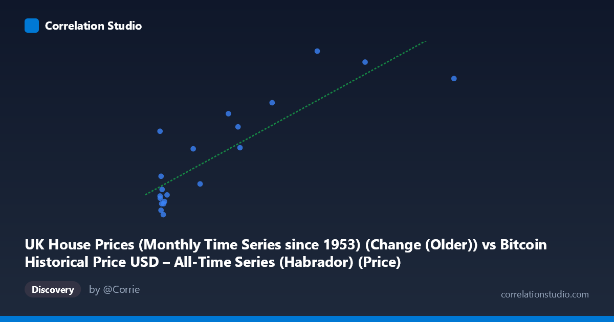
UK House Prices (Monthly Time Series since 1953) (Change (Older)) vs Bitcoin Historical Price USD – All-Time Series (Habrador) (Price)
- Pearson correlation (r)
- 0.8528
- Spearman correlation
- 0.6987
- p-value
- 0.000002
- Sample size (n)
- 20
- 95% confidence interval
- 0.659 to 0.9404
- Granger causality
- None
- Granger optimal lag
- 5
AI analysis
Analysis of Scatterplot Relationship
1. Overview of the Relationship
The scatterplot displays a clear positive, roughly linear relationship between the X variable (labeled here as UK House Prices but evidently mismatched with Bitcoin-scale values) and Y (labeled Bitcoin Price but showing small values consistent with a "change" metric). As X increases from near-zero to over 850, Y rises correspondingly from negative/near-zero values to a maximum of 13.40. The regression line (y = 0.0172x + 1.042) captures this upward trend reasonably well, though the scatter around the line grows more pronounced at higher X values, suggesting mild heteroscedasticity.
2. Strength, Direction, and Statistical Confidence
The correlation is strong and positive (r = 0.853), with r² = 0.727 indicating that approximately 73% of the variance in Y is statistically explained by X — a substantial share, leaving about 27% attributable to other factors or noise. The 95% confidence interval [0.659, 0.940] is reasonably tight and entirely positive, and the p-value (1.78E-06) is highly significant, giving strong confidence that this correlation is not due to chance in this sample. However, the Granger causality test tells a different story: neither direction shows significant predictive causality (X→Y: p=0.133; Y→X: p=0.848). This is a critical distinction — correlation without Granger causality suggests the two series move together contemporaneously (or share a common driver/trend) but neither reliably predicts the other's future values at the tested lag structure (5 periods). This is common with two variables that are both trending over time without a direct causal mechanism linking them.
3. Notable Patterns and Outliers
Several features stand out: near X=0 there's an interesting outlier where Y=6.10 despite X being only 0.06 — far above what the regression would predict, suggesting an anomaly or a point from a different regime. Most low-X points (X<20) cluster near Y=0, with some slightly negative Y values (-0.3 to -1.5), indicating noise or minor declines dominate at small X. The high-X points (X450) show consistently high Y values (10.9–13.4), reinforcing the trend but with only 3-4 points anchoring this upper region — meaning the strength of the linear fit is disproportionately influenced by a handful of high-leverage observations.
4. Confounding Factors and Caveats
The variable labeling is suspicious: X is described as "UK House Prices" but ranges up to 853 (inconsistent with monthly UK house price changes, which are typically small percentages), while Y is labeled "Bitcoin Price" but ranges only -1.5 to 13.4 (inconsistent with actual Bitcoin USD prices, which have spanned thousands of dollars). This strongly suggests axis mislabeling or a metadata mismatch — likely these are actually reversed, transformed, or scaled versions of the described columns. Additionally, both Bitcoin prices and house prices are highly autocorrelated time series with long-term upward trends over 2010–2015; two unrelated trending series can produce spurious high correlation (a classic time-series pitfall). The small sample size (n=20 paired points vs. N=290 population) also limits robustness — outliers can have outsized leverage on r and the regression slope.
5. Recommendations for Further Investigation
Given the axis/label confusion, the first step should be verifying and correcting the data source mapping before drawing substantive conclusions. Assuming the relationship is genuine, analysts should: (a) test for spurious correlation by differencing both series (analyzing returns/changes rather than levels) to remove shared trend effects, (b) increase the sample size beyond 20 points to better estimate the true relationship and reduce outlier sensitivity, (c) explore non-linear or lagged relationships beyond the 5-period Granger test, and (d) investigate potential confounding macroeconomic variables (e.g., inflation, monetary policy, or global risk sentiment) that could simultaneously drive both housing prices and Bitcoin valuations without one directly causing the other.
X dataset: Bitcoin Historical Price USD – All-Time Series (Habrador)
Y dataset: UK House Prices (Monthly Time Series since 1953)
Part of experiment: Bitcoin - Bitcoin Historical Price USD – All-Time Series (Habrador) vs UK House Prices (Monthly Time Series since 1953)